In economics, equilibrium is the cornerstone for understanding how markets operate and reach stability. When an economy reaches equilibrium, supply and demand balance each other across markets, and no further changes are required unless external factors disrupt the balance. Economists have developed two critical methods for analyzing equilibrium: general equilibrium and partial equilibrium. While partial equilibrium focuses on isolated markets, general equilibrium considers the entire economic system.
This article provides a comprehensive guide to both approaches. We will explore their theoretical foundations, key contributors, mathematical formulations, and the ongoing debates about their relevance in modern economics. We will also discuss Walras’ Law, the Arrow‑Debreu model, and the limitations that have spurred further research. By the end, you will understand why these frameworks remain central to economic analysis and how they complement each other.
What Is Equilibrium in Economics?
In economic terms, equilibrium occurs when the quantity of goods demanded by consumers equals the quantity supplied by producers. At this point, there is no incentive for price changes, and the market “clears.” This condition can be analyzed in isolation (partial equilibrium) or as part of a broader system (general equilibrium).
Equilibrium is not merely a theoretical construct; it underpins how we understand price formation, resource allocation, and the effects of policy interventions. Whether we are studying a single commodity market or the entire economy, the concept of equilibrium provides a benchmark against which we can measure deviations and analyze adjustments.
General Equilibrium
General equilibrium theory seeks to explain how supply and demand simultaneously balance across all markets in an economy. Rather than examining individual markets in isolation, general equilibrium takes a holistic approach by considering the interactions between multiple markets. This allows economists to understand how shocks in one market, such as a rise in oil prices, ripple through the economy, affecting other markets like transportation, manufacturing, and consumer spending.
In general equilibrium, we assume that all economic agents (consumers and firms) act to maximize their utility or profit. Prices adjust so that all markets simultaneously reach equilibrium, where supply equals demand across the board.

Figure 1 illustrates a stylised general equilibrium where the intersection of market and firm curves represents the point where supply equals demand in all markets simultaneously. In a full general equilibrium model, this balance occurs across multiple interconnected markets.
Historical Foundations: Léon Walras
The origins of general equilibrium theory trace back to Léon Walras, a French economist of the late 19th century. In his seminal work Éléments d’économie politique pure (1874), Walras set out to demonstrate that an economy of many markets could achieve a consistent set of prices where all markets clear. He used a system of simultaneous equations to represent demand and supply for each good, and he introduced the concept of tâtonnement (groping) to describe how prices adjust toward equilibrium.
Walras’ vision was revolutionary: it shifted economics from the study of isolated markets to the study of the economy as an interdependent system. However, he lacked the mathematical tools to prove that such an equilibrium always exists, a challenge that would be taken up by later economists.
Understanding General Equilibrium Through Mathematical Modeling
General equilibrium is often modeled using a system of equations that captures the behavior of consumers and firms across multiple markets. In its simplest form, for a market with two goods (good X and good Y), general equilibrium can be represented as:
Demand for good X = Supply of good X
Demand for good Y = Supply of good Y
In more advanced models, like the Arrow‑Debreu general equilibrium model, the economy is described by:
- Demand equations for each good represent how much consumers want to buy based on prices and income.
- Supply equations for each good, showing how much firms are willing to produce based on production costs and technology.
- Price equations that adjust to clear each market, meaning that for every good, supply equals demand.
In these models, equilibrium is reached when prices and quantities in all markets simultaneously balance, ensuring that no excess supply or demand exists. The market‑clearing condition can be expressed mathematically as:
where \( x_i(p) \) represents consumer demand, \( y_j(p) \) represents firm supply, and \( p \) denotes the price vector. \( N \) and \( M \) are the number of consumers and firms, respectively. This set of equations adjusts to find prices that clear all markets simultaneously, reflecting the interdependence of the economy.
The Arrow‑Debreu Model of General Equilibrium
The Arrow‑Debreu model, developed by Kenneth Arrow and Gérard Debreu in the 1950s, is the most famous formalization of general equilibrium. It was built on Walras’ intuition by providing rigorous mathematical proof of the existence of equilibrium under specific assumptions. The model assumes:
- Perfect competition: All agents are price‑takers.
- Complete markets: Every possible good (including future goods) has a market with a price.
- Rational agents: Consumers maximise utility; firms maximise profits.
- Convex preferences and production sets.
Under these assumptions, Arrow and Debreu proved that a general equilibrium exists. Moreover, they showed that such an equilibrium is Pareto efficient, a result that connects general equilibrium to the fundamental theorems of welfare economics. The Arrow‑Debreu model remains the benchmark for general equilibrium theory, though it is often criticised for its restrictive assumptions.
Existence, Uniqueness, and the Sonnenschein‑Mantel‑Debreu Theorem
A key aspect of general equilibrium theory is the existence and uniqueness of equilibrium. Existence can be proven under standard assumptions (convexity, completeness, etc.). However, uniqueness is far from guaranteed. The Sonnenschein‑Mantel‑Debreu theorem (1970s) demonstrated that the excess demand functions derived from general equilibrium models can take almost any shape consistent with a few basic properties (continuity, homogeneity, and Walras’ Law). This means that, in general, there is no reason to expect a unique equilibrium; multiple equilibria may exist, and the economy could settle into different outcomes depending on initial conditions or expectations.
This result has profound implications. It means that comparative statics (analyzing how the equilibrium changes with parameters) cannot be reliably performed without additional restrictions. Economists have since explored conditions under which uniqueness holds, such as gross substitutes or specific functional forms, but the general case remains open.
Stability and the Tâtonnement Process
Stability concerns how an economy adjusts after a shock. Walras’ tâtonnement process (also called the “groping” process) describes a hypothetical adjustment mechanism: an auctioneer calls out prices, agents state their desired trades, and prices are adjusted upward for goods with excess demand and downward for goods with excess supply. No actual trades occur until equilibrium prices are found.
In such a process, equilibrium is stable if small deviations trigger price adjustments that return the system to equilibrium. The stability of tâtonnement depends on the properties of excess demand functions. The Sonnenschein‑Mantel‑Debreu theorem also implies that tâtonnement may not converge globally; cycles or chaos can occur. In reality, markets do not operate with a central auctioneer, and trades often happen at disequilibrium prices, making the adjustment process even more complex.
Partial Equilibrium
While general equilibrium considers the entire economy, partial equilibrium narrows the focus to a single market. Alfred Marshall, in his Principles of Economics (1890), developed this method, which assumes that changes in one market do not affect others. Partial equilibrium analysis helps understand how changes in supply or demand in one market (like the wheat market) affect the price and quantity of that specific good.

Figure 2 shows the standard supply‑and‑demand diagram for a single market. The intersection (E) represents the partial equilibrium price and quantity where quantity demanded equals quantity supplied.
Alfred Marshall and the Ceteris Paribus Assumption
Marshall’s innovation was the ceteris paribus (all else equal) assumption. By holding everything else constant, he could isolate the effect of a single change in a single market. This approach made economic analysis tractable and became the foundation of microeconomics.
For example, suppose wheat prices rise due to a bad harvest. Partial equilibrium analysis helps us understand how this price change affects wheat demand, assuming that other factors, such as wages, fuel prices, or the demand for other crops, remain constant. The result is a clear prediction: a higher price reduces quantity demanded along the demand curve.
Applications and Limitations
Partial equilibrium is widely used in microeconomics to study topics like taxation, subsidies, price controls, and industry regulation. Its strength lies in its simplicity and focus. However, it may miss important feedback effects from other markets. For instance, a tax on sugar might reduce sugar consumption, but it could also affect the market for corn syrup, labor markets in agriculture, and public health outcomes. General equilibrium would capture these, while partial equilibrium would not.
Walras’ Law and Market Interdependence
A critical insight from general equilibrium theory is Walras’ Law, which states that if all but one market in an economy is in equilibrium, the last market must also be in equilibrium. This underscores the interconnectedness of markets. According to Walras’ Law, a shortage or surplus in one market must be balanced by a corresponding shortage or surplus elsewhere in the economy.
Example: Consider a scenario where there is an excess supply of labor in the job market (i.e., unemployment). According to Walras’ Law, this excess supply must be offset by excess demand in another market, perhaps for goods and services. This suggests that imbalances in one area of the economy will be reflected elsewhere, a crucial insight for policymakers.
Analyzing Changes in Equilibrium
In addition to understanding equilibrium, economists study comparative statics, which analyzes how changes in external conditions affect equilibrium. For instance, how does a tax on carbon emissions affect the overall equilibrium in the energy and consumer goods markets? General equilibrium analysis helps answer these questions by considering all markets simultaneously.
Comparative statics can reveal unintended consequences. A subsidy for renewable energy might lower electricity prices, but if it is funded by a tax on labor, it could reduce employment. A general equilibrium approach captures such trade‑offs, while a partial equilibrium analysis might miss them. However, the Sonnenschein‑Mantel‑Debreu theorem shows that without strong restrictions, the sign of comparative statics effects cannot be predicted theoretically; they must be estimated empirically.
Criticisms and Limitations of General Equilibrium Theory
While general equilibrium theory provides a comprehensive framework for understanding market interdependence, it is not without its criticisms:
Perfect Competition
General equilibrium models often assume perfect competition, meaning firms are price takers with no market power. However, in the real world, many industries exhibit monopolistic or oligopolistic behavior, where firms have significant control over prices.
Complete Markets
Assuming all markets exist and are complete (i.e., every good or service has a market) is highly unrealistic. Many real‑world markets, like healthcare or education, have incomplete information or are heavily regulated, leading to inefficiencies.
Rationality and Information
General equilibrium assumes that all agents have perfect information and act rationally to maximize utility. In practice, information asymmetry and irrational behavior often lead to market failures.
Real‑World Frictions
Transaction costs, taxes, and regulations can distort markets, making it difficult for economies to achieve general equilibrium. Moreover, the tâtonnement process assumes that no trades occur until equilibrium prices are found, which is not how actual markets work.
Multiple Equilibria and Indeterminacy
As the Sonnenschein‑Mantel‑Debreu theorem shows, multiple equilibria are possible, and the economy may not converge to a unique outcome. This makes policy analysis less straightforward.
Despite these limitations, general equilibrium remains a powerful benchmark for thinking about the economy as a whole, and modern extensions (e.g., incorporating imperfect competition, asymmetric information, or behavioral biases) continue to build on its foundations.
General vs. Partial Equilibrium
| Aspect | General Equilibrium | Partial Equilibrium |
|---|---|---|
| Scope | Entire economy and multiple markets | Single market studied in isolation |
| Interdependence | Considers how changes in one market affect others | Ignores other markets, assumes they remain constant |
| Methodology | Complex, requires advanced mathematical models | Simpler, uses supply‑and‑demand diagrams |
| Key Figures | Léon Walras, Arrow‑Debreu | Alfred Marshall |
| Assumptions | Perfect competition, complete markets, convexity | Ceteris paribus, no spillovers |
| Applications | Tax policy, trade, climate policy, financial crises | Industry analysis, excise taxes, price controls |
| Advantages | Captures feedback effects, theoretically rigorous | Easy to apply, intuitive |
| Limitations | Computationally demanding, restrictive assumptions | May miss important interactions |

|
||
Extensions and Modern Developments
Modern economics has extended both frameworks to address their limitations:
- Imperfect competition has been integrated into general equilibrium models (e.g., models with monopolistic competition).
- Incomplete markets are now studied using models with borrowing constraints, asymmetric information, and transaction costs.
- Behavioral economics incorporates bounded rationality into equilibrium analysis.
- Computable general equilibrium (CGE) models allow empirical analysis of policies (e.g., trade agreements, carbon taxes) by calibrating models to real data.
- Dynamic general equilibrium models (e.g., DSGE) incorporate time and uncertainty, forming the backbone of modern macroeconomics.
These developments have made equilibrium analysis more realistic while preserving its core insights.
Conclusion
Both general and partial equilibrium analyses provide valuable insights into how markets function and reach stability. While general equilibrium offers a holistic view of the entire economy, partial equilibrium allows economists to study individual markets in isolation. Each has its strengths and limitations; understanding both is essential for analyzing complex economic systems.
Economists continue to build on these foundational theories, refining them to better account for real‑world complexities, such as information asymmetry, market frictions, and monopolistic competition. By understanding how markets reach equilibrium, we gain a deeper understanding of economic dynamics, helping policymakers design better interventions for societal welfare.
FAQs:
What is equilibrium in economics?
In economics, equilibrium occurs when the quantity of goods demanded by consumers equals the quantity supplied by producers. At this point, market prices stabilize, and no further changes in supply or demand occur unless external factors disrupt the balance.
What is general equilibrium analysis?
General equilibrium analysis looks at the entire economy, considering the interactions and interdependencies between multiple markets. It examines how equilibrium is achieved when supply and demand balance across all markets simultaneously, considering the ripple effects that changes in one market can have on others.
What is partial equilibrium analysis?
Partial equilibrium analysis focuses on a single market in isolation, assuming that other markets remain constant. This approach simplifies the analysis by concentrating on the effects of supply and demand within one market, without considering interactions with other markets.
How does general equilibrium differ from partial equilibrium?
General equilibrium considers the entire economy, including the interrelationships between multiple markets, while partial equilibrium isolates one market, assuming that other markets remain unaffected. General equilibrium uses more complex mathematical models, whereas partial equilibrium is simpler and commonly used in microeconomic studies.
What is Walras’ Law?
Walras’ Law states that if all but one market in an economy is in equilibrium, the final market must also be in equilibrium. It highlights the interconnectedness of markets and suggests that surpluses or shortages in one market must be offset by imbalances in other markets.
What is the Arrow-Debreu model of general equilibrium?
The Arrow-Debreu model formalizes the concept of general equilibrium in a competitive economy. It assumes rational consumers, firms, and complete markets, and mathematically demonstrates that under certain conditions, an equilibrium exists where no agent can improve their utility without making someone else worse off.
What are the advantages of using general equilibrium analysis?
General equilibrium analysis provides a holistic view of the economy by showing how changes in one market affect others. This is particularly useful for analyzing broad economic policies, trade, and systemic shocks that impact multiple sectors simultaneously.
What are the limitations of general equilibrium theory?
General equilibrium theory often assumes perfect competition, complete markets, and rational behavior, which are not always realistic. It also overlooks real-world frictions like transaction costs, taxes, and regulations, which can prevent markets from achieving equilibrium in practice.
When is partial equilibrium analysis more appropriate?
Partial equilibrium analysis is more appropriate when analyzing the effects of changes in one specific market without needing to consider how other markets are affected. It is particularly useful for studying microeconomic issues, such as taxation or price changes in individual markets.
What is the role of comparative statics in general equilibrium analysis?
Comparative statics examines how changes in external factors, such as taxes or technological innovations, affect the equilibrium in various markets. It allows economists to predict how a new policy or external event will shift the overall economic equilibrium.
Thanks for reading! Share this with friends and spread the knowledge if you found it helpful.
Happy learning with MASEconomics