In economics and social sciences, understanding relationships between variables is essential to uncover patterns, make predictions, and guide decision-making. Econometric models help researchers analyze these relationships In economics and social sciences, many real-world phenomena involve qualitative outcomes, such as whether a customer buys a product, an individual votes, or a patient tests positive for a disease. Traditional regression models like Ordinary Least Squares (OLS) are unsuitable for analyzing such binary outcomes.
Binary choice models, such as the logit and probit models, address this need by estimating the probability of an event occurring based on explanatory variables. These models are widely applied in areas like voting behavior, health outcomes, and consumer choices, making them essential tools in econometrics.
What are Qualitative Dependent Variables?
In econometrics, a dependent variable represents the outcome we aim to analyze or predict. When this variable takes on categorical values instead of continuous numerical values, it is referred to as a qualitative dependent variable.
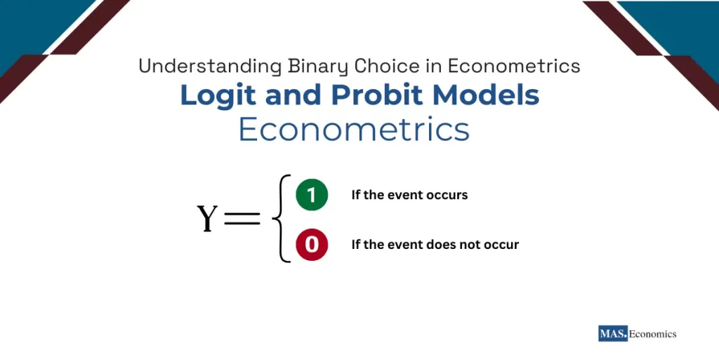
The most common type of qualitative dependent variable is binary, where the outcome has only two categories:
Examples of Binary Dependent Variables:
- Voting Behavior: Did the person vote? (Yes/No)
- Health Outcomes: Was the test positive? (Positive/Negative)
- Customer Choices: Did the customer buy the product? (Buy/Don’t Buy)
Traditional OLS regression models assume a continuous dependent variable and fail to provide meaningful results for binary outcomes. The predicted probabilities can exceed the logical bounds of 0 and 1, leading to invalid interpretations.
To address this, economists use logit and probit models, which are specifically designed to handle binary dependent variables while ensuring the predicted probabilities remain between 0 and 1.
Understanding Logit Models
The logit model, also known as logistic regression, is one of the most widely used tools for analyzing binary outcomes. It estimates the probability of a particular event occurring, such as whether a customer will purchase a product, a patient will develop a disease, or a voter will cast their vote.
The logit model solves a key limitation of traditional regression models (like OLS) when dealing with binary dependent variables: the risk of predicted probabilities exceeding the bounds of 0 and 1. To avoid this, the logit model transforms probabilities using the logistic function, ensuring predictions remain within logical limits.
The Logistic Transformation
The logistic function takes the form:
Here:
- \( P(Y = 1) \): Probability of the event occurring.
- \( \beta_0 \): Intercept term.
- \( \beta_1, \dots, \beta_k \): Coefficients of the independent variables \( X_1, X_2, \dots \).
- \( e \): Euler’s number, approximately 2.718.
The logistic function produces an S-shaped curve, where the probability of \( Y = 1 \) increases non-linearly as the independent variables increase. This transformation ensures that the estimated probabilities stay between 0 and 1.
The Log-Odds Interpretation
The logit model estimates the relationship between the independent variables and the log-odds (or logit) of the outcome:
The log-odds represent the natural logarithm of the odds ratio. The odds ratio, in turn, is defined as the ratio of the probability that an event occurs to the probability that it does not:
- If \( \beta_1 > 0 \), an increase in \( X_1 \) increases the log-odds (and thus the probability) of \( Y = 1 \).
- If \( \beta_1 < 0 \), an increase in \( X_1 \) decreases the log-odds.
While log-odds are less intuitive than raw probabilities, they provide a linear relationship that is easy to model mathematically.
Why Use the Logit Model?
The logit model has several advantages:
- Logical Probabilities: The logistic function ensures that all predicted probabilities fall between 0 and 1.
- Flexibility: It can handle various types of independent variables (e.g., continuous, categorical).
- Interpretability: While log-odds may seem complex, they can be easily transformed into odds ratios, which are widely used in fields like health and business.
Practical Example: Predicting Customer Purchase
Suppose a company wants to determine the likelihood that a customer purchases a product based on:
- \( X_1 \): Product price.
- \( X_2 \): Advertising spend.
- \( X_3 \): Customer income.
The logit model might yield the following equation:
- A negative coefficient on price (\(-0.2\)) means that higher prices reduce the odds of purchase.
- A positive coefficient on advertising spend (0.5) means that increased advertising raises the odds of purchase.
By plugging in specific values of \( X_1, X_2, \) and \( X_3 \), the company can calculate the probability of purchase for any given customer.
Exploring Probit Models
The probit model is another popular approach for binary choice problems. Like the logit model, it estimates the probability of an event occurring, but it assumes that the error terms follow a normal distribution instead of a logistic distribution.
The Probit Function
The probit model expresses the probability of \( Y = 1 \) as a function of the cumulative distribution function (CDF) of the standard normal distribution:
Where \( \Phi \) is the CDF of the standard normal distribution.
This function maps the linear combination of the independent variables (\( \beta_0 + \beta_1 X_1 + \dots \)) to a probability value between 0 and 1. The resulting curve is also S-shaped but arises from the normal distribution rather than the logistic distribution.
Key Differences from the Logit Model
While the logit and probit models look similar, they differ in how they model the probabilities:
- Logit: Uses the logistic function, which assumes slightly heavier tails in the distribution.
- Probit: Uses the normal CDF, which assumes thinner tails.
This difference in tail behavior can affect results when dealing with extreme probabilities (very close to 0 or 1). However, in most practical applications, the results of the two models are very similar.
Why Use the Probit Model?
The probit model is preferred when:
- The assumption of normally distributed errors aligns better with the underlying theory.
- The dataset is small, and normality assumptions help improve the model’s precision.
Practical Example: Health Outcomes Analysis
Suppose researchers are studying the probability of testing positive for a disease based on:
- \( X_1 \): Age.
- \( X_2 \): Lifestyle habits (e.g., smoking).
- \( X_3 \): Family history.
The probit model provides a probability estimate based on the standard normal CDF, ensuring that the probabilities are logically constrained between 0 and 1. For example:
- Older age and family history might significantly increase the likelihood of a positive test.
- A healthier lifestyle might reduce this likelihood.
Logit vs. Probit: Key Differences
After understanding the individual mechanics of logit and probit models, it is essential to compare them directly to highlight their unique characteristics. Below is a table summarizing the key distinctions:
| Aspect | Logit Model | Probit Model |
|---|---|---|
| Error Distribution | Logistic distribution | Normal distribution |
| Probability Curve | Logistic function (heavier tails) | Normal CDF (thinner tails) |
| Computational Simplicity | Easier to compute | More complex computation |
| Interpretation | Produces log-odds ratios | Produces probabilities directly |
| Theoretical Justification | Widely used due to flexibility | Preferred when normality is assumed |

|
||
While logit models are more popular due to their simplicity and ease of interpretation, probit models offer theoretical advantages in cases where normality is justified.
Having understood the theoretical distinctions between logit and probit models, let’s explore their practical uses across different fields to see how these tools are applied in real-world scenarios.
Applications of Logit and Probit Models
Logit and probit models are versatile tools applied across various fields to analyze binary outcomes. Below are their applications in key areas:
Election Analysis and Voter Behavior
Political analysts use these models to predict voter turnout and understand electoral behavior. Variables such as education, income, and exposure to political campaigns influence voting decisions. For example, a probit model might estimate the likelihood of turnout among citizens targeted by a political outreach campaign. These insights help design strategies to engage voters effectively.
Predicting Health Outcomes
Healthcare researchers frequently apply probit models to study disease risk and treatment efficacy. Variables like age, lifestyle choices, and preventive measures such as vaccination are analyzed to determine the likelihood of specific health outcomes. By identifying high-risk populations, policymakers can design targeted interventions and improve public health programs.
Consumer Choice in Marketing
Businesses rely on logit models to understand customer purchasing behavior. Factors such as price sensitivity, advertising campaigns, and product features determine whether a customer will buy a product. For instance, a logit model might help a retailer evaluate how promotional discounts affect purchase likelihood, enabling data-driven marketing decisions.
Credit Risk Assessment
In finance, logit models are used to predict loan default probabilities based on factors like income, credit scores, and loan size. These models provide critical insights for lenders, helping them assess creditworthiness and manage risk effectively.
Why These Applications Matter
The versatility of logit and probit models lies in their ability to handle binary outcomes across different fields. From voter behavior and health outcomes to financial risk and consumer choices, these models provide actionable insights for researchers, policymakers, and businesses alike.
Conclusion
Logit and probit models are essential tools in econometrics for analyzing binary outcomes, providing a reliable framework for estimating probabilities within the valid range of 0 to 1.
The logit model is often favored for its simplicity and computational ease, while the probit model proves effective when normality assumptions are crucial, especially in smaller samples. Both models have practical applications in fields like voter behavior, health analysis, and consumer choice, offering researchers and analysts robust methods for examining qualitative data with precision.
FAQs
What are logit and probit models?
Logit and probit models are econometric tools used to analyze binary outcomes, such as whether an event occurs or not. They estimate probabilities based on explanatory variables, ensuring the results remain between 0 and 1.
Why are traditional regression models unsuitable for binary outcomes?
OLS regression models assume continuous dependent variables and can produce predicted probabilities outside the logical range of 0 and 1. This makes them unreliable for analyzing binary outcomes like Yes/No or Success/Failure.
How does the logit model work?
The logit model uses the logistic function to transform probabilities into a log-odds scale. This ensures the predicted probabilities stay within 0 and 1. It is particularly useful for interpreting relationships as odds ratios.
What is the probit model?
The probit model uses the cumulative distribution function (CDF) of the standard normal distribution to estimate probabilities. It assumes that the error terms follow a normal distribution, making it suitable for applications where this assumption aligns with the data.
How do logit and probit models differ?
Logit models use a logistic function with heavier tails, while probit models rely on the normal distribution’s CDF with thinner tails. In most applications, their results are similar, but probit models are preferred when normality is assumed.
What are the applications of logit and probit models?
Logit and probit models are used in voter behavior analysis to predict turnout and election outcomes, in healthcare to estimate disease risk or treatment success, in marketing to analyze customer purchase decisions, and in finance to assess credit risk and loan default probabilities.
When should I use a logit model instead of a probit model?
Use the logit model for simplicity and ease of interpretation, particularly when odds ratios are required. Choose the probit model when the error terms are assumed to follow a normal distribution or when working with small samples.
Thanks for reading! Share this with friends and spread the knowledge if you found it helpful.
Happy learning with MASEconomics


