A development economist evaluating a cash transfer program in rural Kenya faces a familiar problem. Three small randomized trials have produced point estimates that bounce around: one shows a 12% income gain, another 4%, and a third 18%. The frequentist toolkit returns a wide confidence interval and a p-value that may or may not clear 0.05. Policymakers want a different answer entirely. They want to know the probability that the program actually works, and by how much. Bayesian econometrics answers exactly that question. It combines existing knowledge with new data and produces probability statements about parameters that frequentist methods, by construction, cannot deliver.
The shift in thinking is fundamental. A frequentist 95% confidence interval does not say there is a 95% probability the true effect lies inside it. It says that if the experiment were repeated infinitely many times, 95% of such intervals would contain the true value. A Bayesian credible interval says what most people thought a confidence interval said in the first place: given the data and prior beliefs, there is a 95% probability the parameter lies inside this range. That difference matters when decisions have to be made under uncertainty, which is most of the time in applied economics.
What Bayesian Methods Solved
The core problem in econometrics is moving from data to beliefs about parameters. A coefficient on schooling in a wage regression, the elasticity of demand for electricity, and the persistence of a monetary policy shock, all these are all quantities researchers want to learn about. The frequentist framework treats parameters as fixed, unknown constants and data as random. Probability statements attach to procedures, not to parameters themselves. The Bayesian framework reverses this. Parameters are treated as random variables with probability distributions that represent uncertainty, and data are treated as observed facts that update those distributions.
This reversal solves a problem that has bothered applied economists for decades. Suppose a new study estimates the elasticity of intertemporal substitution at 0.4, with a standard error of 0.3. Twenty previous studies have produced estimates clustered tightly around 0.5. A frequentist analysis of the new study gives a wide confidence interval that ignores the prior literature. A Bayesian analysis combines the prior evidence with the new data and produces a posterior distribution that reflects both. The result is sharper inference and a natural way to accumulate knowledge across studies.
Bayesian thinking also dissolves several puzzles that vex frequentist practice. The garden of forking paths, the multiple comparisons problem, and the difficulty of stopping rules in sequential experiments all become more tractable when probability is interpreted as a degree of belief. A researcher who runs an experiment, looks at interim data, and decides whether to continue is not violating Bayesian principles. The posterior simply reflects whatever data have been observed, regardless of why the researcher chose to stop.
Three forces have pushed Bayesian methods from a philosophical curiosity in the 1950s to a workhorse in modern applied economics. First, computational advances, particularly Markov Chain Monte Carlo, made posterior distributions tractable for realistic models. Second, hierarchical models for panel data, meta-analysis, and small-area estimation turned out to be naturally Bayesian. Third, software like Stan, PyMC, and JAGS lowered the cost of entry from years of programming to a few weeks of learning.
Bayes’ Rule in Equations
The mathematical core of Bayesian inference is a single equation that follows from the definition of conditional probability. For a parameter \( \theta \) and data \( y \), Bayes’ theorem states:
The left-hand side is the posterior distribution, the object of interest. The numerator has two pieces. The likelihood \( p(y \mid \theta) \) describes how probable the observed data are for each possible value of \( \theta \). The prior \( p(\theta) \) encodes beliefs about \( \theta \) before seeing the data. The denominator \( p(y) \) is the marginal likelihood, a normalizing constant that ensures the posterior integrates to one. Because \( p(y) \) does not depend on \( \theta \), the posterior is often written in proportional form:
This compact expression captures the essence of Bayesian updating. The posterior is proportional to the prior times the likelihood. New data reweight prior beliefs in proportion to how well each parameter value explains what was observed.
The normal-normal conjugate model gives the cleanest worked example. Suppose a researcher wants to estimate the mean \( \theta \) of a population with known variance \( \sigma^2 \). The prior belief is that \( \theta \) follows a normal distribution centered at \( \mu_0 \) with variance \( \tau_0^2 \):
A sample of \( n \) observations with mean \( \bar{y} \) is collected, where each observation is normally distributed around \( \theta \) with variance \( \sigma^2 \). The likelihood is:
Multiplying the prior by the likelihood and completing the square gives a posterior that is itself normal:
where the posterior mean and variance are:
The posterior mean \( \mu_n \) is a precision-weighted average of the prior mean \( \mu_0 \) and the sample mean \( \bar{y} \). Precision is the inverse of variance. As the sample size grows, the data precision \( n/\sigma^2 \) overwhelms the prior precision \( 1/\tau_0^2 \), and the posterior converges to the maximum likelihood estimate. With small samples or strong priors, the posterior leans toward the prior. This shrinkage behavior is one of the reasons Bayesian estimators often outperform frequentist alternatives in finite samples.
Most realistic models do not have closed-form posteriors. The likelihood may involve nonlinear functions of many parameters, the prior may not be conjugate, and the integral that defines the marginal likelihood may be intractable. Markov Chain Monte Carlo solves this problem by generating samples from the posterior without computing the normalizing constant. The Metropolis-Hastings algorithm proposes a new parameter value, computes the ratio of posterior densities at the proposed and current values, and accepts the proposal with a probability that depends on this ratio. The Gibbs sampler is a special case that cycles through full conditional distributions one parameter at a time. Hamiltonian Monte Carlo, the engine behind Stan, uses gradient information to propose moves that travel further across the posterior with higher acceptance rates.
The output of MCMC is a sequence of parameter draws \( \theta^{(1)}, \theta^{(2)}, \ldots, \theta^{(M)} \) whose empirical distribution approximates the posterior. Posterior means, medians, credible intervals, and probabilities of any statement about the parameters can be computed by summarizing these draws.

| Symbol | Meaning |
|---|---|
| \( \theta \) | Parameter or vector of parameters of interest |
| \( y \) | Observed data |
| \( p(\theta) \) | Prior distribution, beliefs about \( \theta \) before seeing data |
| \( p(y \mid \theta) \) | Likelihood, probability of data given \( \theta \) |
| \( p(\theta \mid y) \) | Posterior distribution, beliefs about \( \theta \) after seeing data |
| \( p(y) \) | Marginal likelihood, normalizing constant |
| \( \mu_0, \tau_0^2 \) | Prior mean and variance in the normal-normal model |
| \( \mu_n, \tau_n^2 \) | Posterior mean and variance after \( n \) observations |
| \( \bar{y} \) | Sample mean of observed data |
| \( \sigma^2 \) | Known variance of the data-generating process |
| \( \theta^{(m)} \) | The \( m \)-th draw from an MCMC chain targeting the posterior |
| \( \hat{R} \) | Gelman-Rubin convergence diagnostic for MCMC chains |
 | |
Table 1. Notation Used in Bayesian Econometrics: Symbols and Definitions
Assumptions of Bayesian Methods
Bayesian inference rests on assumptions that deserve scrutiny. The most prominent is the prior. Every Bayesian analysis requires a prior distribution for every parameter, and that choice influences the posterior. With informative priors and small samples, the prior can dominate the data. Critics of Bayesian methods point to this as a source of subjectivity that has no place in scientific inference. Defenders respond that frequentist analysis also embeds assumptions, often implicit ones, in functional forms and model specifications, and that an explicit prior is more honest than a hidden one.
Prior sensitivity analysis is the practical response. A well-conducted Bayesian study reports results under several priors: a weakly informative default, an informative prior based on previous literature, and a skeptical prior that pushes against the hypothesis being tested. If the substantive conclusions are stable across these specifications, prior sensitivity is not a serious concern. If conclusions flip, the analysis is honestly reporting that the data alone cannot decide the question.
The choice between subjective and objective priors is a long-standing debate. Subjective Bayesians argue that priors should reflect genuine prior knowledge, including expert judgment. Objective Bayesians prefer reference priors, Jeffreys priors, or other rules that aim for minimal information content. In practice, applied economists often use weakly informative priors that encode mild constraints, such as ruling out absurdly large effects, while letting the data drive most of the posterior.
Computational cost is the second major limitation. Fitting a Bayesian model with MCMC can take hours or days for complex hierarchical models, while a frequentist regression runs in seconds. Modern variational inference and Hamiltonian Monte Carlo have reduced this gap, but it has not closed entirely. For routine applied work with large samples and standard models, the gain from going Bayesian may not justify the extra time.
Convergence diagnostics are non-negotiable. MCMC produces valid posterior samples only if the chain has converged to the target distribution. Standard diagnostics include the Gelman-Rubin statistic \( \hat{R} \), which compares variance within chains to variance between chains and should be close to 1.0; effective sample size, which measures how many independent draws the autocorrelated chain is worth; and trace plots, which should show stationary mixing rather than trends or stuck chains. A Bayesian analysis without convergence checks is uninterpretable, regardless of how sophisticated the model.
Bayesian methods are not always worth the extra effort. With large samples, default priors, and standard linear models, frequentist and Bayesian estimates typically agree to several decimal places. The interpretation differs, but the numbers do not. The case for Bayesian methods strengthens when sample sizes are small, when prior information is genuinely informative, when hierarchical structure matters, when the question of interest is naturally probabilistic, or when decisions must be made under uncertainty rather than hypotheses tested.
Testing Bayesian Inference
Empirical applications of Bayesian methods have multiplied across applied economics. Three areas illustrate the range. In macroeconomic forecasting, Bayesian Vector Autoregressions have become standard tools at central banks. Research at the Federal Reserve has documented how Minnesota-style priors that shrink VAR coefficients toward simple random walks improve forecast accuracy substantially relative to unrestricted VARs. The intuition is straightforward. With dozens of variables and limited time series, unrestricted estimation is noisy. Shrinkage toward economically sensible defaults reduces variance more than it adds bias. Hierarchical Bayesian VARs now form part of the forecasting toolkit at the European Central Bank and the Bank of England.
In education economics, hierarchical Bayesian models have transformed value-added estimation for teachers and schools. Studies by RAND researchers showed that frequentist estimates of teacher effects are noisy when class sizes are small, leading to teachers being unfairly classified as ineffective based on a few unrepresentative students. Hierarchical Bayesian estimators shrink individual teacher effects toward the population means, with the degree of shrinkage determined by the data. The result is more stable rankings, fewer false positives, and better policy decisions.
Development economics has adopted Bayesian methods for meta-analysis of randomized trials. When a question has been studied across multiple contexts, hierarchical models allow researchers to pool information while accounting for heterogeneity. Work synthesizing cash transfer evaluations has shown that posterior distributions for treatment effects are tighter and more honest than naive averages of point estimates. A policymaker reading such an analysis can directly answer questions like “what is the probability that this program will reduce poverty in my country by at least 10 percentage points?”
The contrast between frequentist and Bayesian inference becomes most visible when the same data are analyzed both ways. Consider a small clinical-style economic experiment with a treatment effect estimate of 2.0 and a standard error of 1.2. The frequentist 95% confidence interval runs from -0.35 to 4.35. A Bayesian analysis with a weakly informative prior centered at zero produces a posterior that, while similar in shape, supports direct probability statements: there is roughly an 85% probability that the treatment effect is positive, and a 60% probability it is at least 1.0. These probability statements are exactly what decision makers want to know.
Figure 1. Posterior distribution with 95% credible interval (Bayesian) compared to a frequentist confidence interval for the same data. The Bayesian posterior supports direct probability statements about the parameter; the frequentist interval describes the long-run behavior of the procedure. Source: MASEconomics simulation based on standard normal-normal conjugate analysis.
Bayesian methods have also performed well in horse races against machine learning approaches. In structured economic problems where theory provides guidance about functional forms and reasonable parameter ranges, Bayesian models often match or beat black-box predictors while delivering interpretable uncertainty. The combination of theoretical structure with probabilistic uncertainty quantification is a niche where Bayesian econometrics has clear advantages over both classical regression and modern machine learning.
Bayesian Thinking and Policy
The case for Bayesian econometrics in modern applied work rests on three pillars. The first is decision theory. Most economic policy is not a hypothesis test but a decision under uncertainty. A central bank choosing whether to raise rates, a finance ministry projecting debt sustainability, and a regulator setting capital requirements all face decisions where the relevant question is the expected value of the outcome under each option. Posterior distributions are the natural input to expected-utility calculations. Frequentist confidence intervals and p-values do not plug directly into decision rules without ad hoc translation.
The Bank of England has explicitly framed monetary policy decisions in terms of probabilities derived from forecast distributions. The fan charts published in Inflation Reports show probability bands around inflation projections, computed from models that are essentially Bayesian in spirit. The shift from point forecasts with confidence intervals to probability distributions over outcomes mirrors the conceptual shift from frequentist to Bayesian thinking. Treasury departments in the United States, United Kingdom, Canada, and Australia have moved in similar directions for fiscal projections, presenting ranges of debt-to-GDP outcomes under uncertainty rather than single deterministic forecasts.

The second pillar is software. Stan, developed at Columbia University, lets users specify Bayesian models in a domain-specific language and uses Hamiltonian Monte Carlo to produce posterior samples. The Stan documentation covers everything from linear regression to complex hierarchical and time-series models. PyMC offers similar capabilities in Python, with tighter integration into the scientific Python ecosystem. JAGS and OpenBUGS, while older, still serve well for Gibbs-friendly models. R packages like brms and rstanarm provide formula-style interfaces that make Bayesian regression as easy to write as the frequentist equivalent.
The third pillar is methodology. Bayesian methods integrate naturally with several modern econometric concerns. Hierarchical models for clustered or panel data fall out of the framework directly, without the patchwork of fixed-effects, random-effects, and clustered-standard-error choices that frequentist practice requires. Model averaging across competing specifications becomes a coherent posterior over models rather than a model selection problem. Causal inference benefits when prior knowledge about treatment effects from related contexts can be incorporated formally; researchers familiar with frequentist tools like instrumental variables or multiple regression can extend their workflow with Bayesian variants that handle weak instruments and prior information more gracefully.
Concrete applications in advanced economies show the pattern. The Federal Reserve uses Bayesian DSGE models alongside reduced-form forecasts to inform policy deliberations. Statistics Canada has incorporated hierarchical Bayesian small-area estimation into official labor force statistics, allowing reliable estimates for regions where direct survey samples are too small. The Australian Treasury uses Bayesian methods in modeling tax revenue uncertainty for budget projections. The Office for National Statistics in the United Kingdom employs Bayesian time-series models in producing GDP growth estimates that quantify revision uncertainty.
Applied micro researchers have also found Bayesian methods useful for problems that resist clean frequentist solutions. Structural models with many parameters and limited identification benefit from priors that encode theoretical restrictions softly rather than imposing them as hard constraints. Discrete choice models in industrial organization, where likelihoods can be flat across regions of parameter space, often estimate more reliably with weakly informative priors than with maximum likelihood. Structural equation models and latent variable models, common in development and labor economics, are natural fits for Bayesian estimation.
The connection to other modern tools deserves attention. Bootstrap methods share with Bayesian inference the goal of producing inference without asymptotic approximations, but the bootstrap remains within the frequentist framework and does not deliver direct probability statements about parameters. Causal inference tools like difference-in-differences and regression discontinuity have Bayesian implementations that handle small samples better than their frequentist counterparts and produce posterior distributions over treatment effects that decision makers can use directly.
The intellectual payoff goes beyond technique. Bayesian thinking changes how researchers reason about uncertainty. Instead of asking "would I reject the null at the 5% level?" they ask "given everything I know, how probable is it that this policy will work, and how much should I update if a new study comes out?" That reframing matches how economic decisions actually get made, in central banks, in finance ministries, in development agencies, and in firms. Bayesian econometrics gives that reasoning a rigorous mathematical foundation.
MASEconomics Explains
Four economic concepts behind Bayesian econometrics
Conclusion
Bayesian econometrics offers a coherent framework for combining prior knowledge with new evidence and producing direct probability statements about economic parameters. The approach answers questions that frequentist methods cannot, including the probability that a treatment effect is positive, the probability that inflation will exceed the target, and the probability that a policy will achieve its stated goal. Computational advances and accessible software have removed most of the practical barriers that once limited Bayesian work to specialists. For small samples, hierarchical structures, decision problems, and questions where prior information matters, Bayesian methods often deliver tighter inference and more honest uncertainty quantification than frequentist alternatives. The trade-offs are real, including computational cost, prior sensitivity, and convergence diagnostics, but they are manageable and well understood. Modern applied economics is increasingly Bayesian, and the trend looks likely to continue.
Did you find this article helpful? Share it with someone who loves economics. And remember, at MASEconomics, we make complex ideas simple.