Marginal Rate of Substitution: Slope, Concavity, and Choice

A household weighing whether to spend an extra five dollars on coffee or on tea is doing more than choosing a beverage. It reveals the slope of its indifference curve at the bundle it currently consumes. The marginal rate of substitution measures how much tea the household would willingly give up to obtain one more cup of coffee while keeping its overall satisfaction unchanged. That single number, calculated at every point in the consumption space, is the geometric and behavioural fingerprint of consumer preferences.

Consumer theory rests on three ideas: a preference ordering, a budget constraint, and the point where the two touch. The marginal rate of substitution is what makes that touching point optimal. It equals the slope of the indifference curve at the consumer’s chosen bundle, and at the optimum, it equals the slope of the budget line, which is the price ratio. The conditions that make the MRS well-defined, smooth, and economically meaningful are the foundational assumptions developed in our discussion of the monotonicity, convexity, and differentiability foundations of consumer preferences. This article moves from a concrete example to the formal definition, then to the role of diminishing MRS in delivering interior solutions, and finally to the empirical content the concept carries when researchers move from theory to data.

Coffee, Tea, and the Geometry of Willingness to Substitute

A consumer starts the week with six cups of coffee and four cups of tea. Asked how many cups of tea she would give up to gain a seventh cup of coffee while remaining equally satisfied, she answers one. Asked the same question after she already has nine cups of coffee and one cup of tea, she answers a quarter. The willingness to substitute coffee for tea has fallen as her coffee consumption has risen. This pattern is intuitive: the marginal value of additional coffee declines as the consumer becomes saturated with it, and the marginal value of scarce tea rises as it becomes the smaller share of the bundle.

The geometric translation of that intuition is the slope of an indifference curve. An indifference curve in the coffee-tea plane connects all bundles that give the consumer the same utility. Moving along the curve, gains in coffee are exactly offset by losses in tea. The rate at which tea must be given up for coffee at a point on the curve is the negative of the slope at that point, and that negative slope is the marginal rate of substitution of coffee for tea. The MRS is a local quantity: it depends on where the consumer currently is on the indifference map, not on the entire indifference curve. Our walkthrough of how indifference curves represent consumer behaviour introduces the map; this article focuses on the slope at a single point.

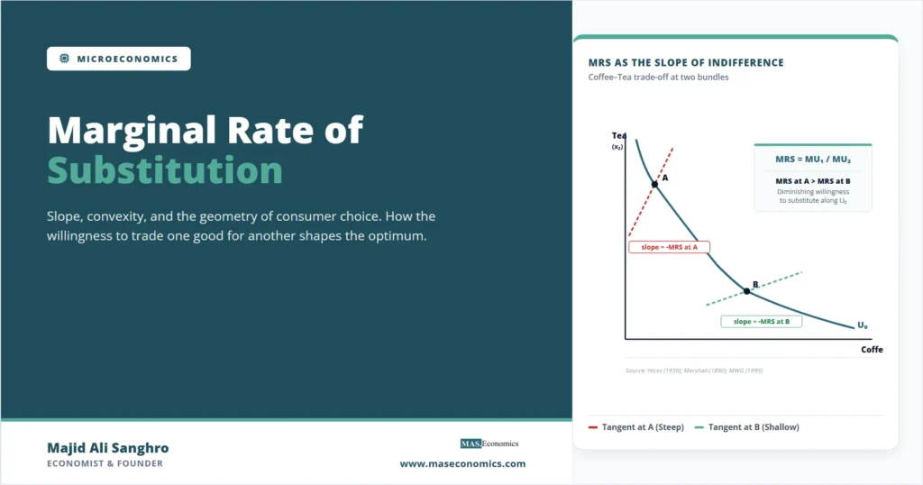
Figure 1. The Marginal Rate of Substitution as the Slope of the Tangent Line: Tea (x₂) Coffee (x₁) U₀ slope = -MRS at A A (low coffee, high tea) slope = -MRS at B B (high coffee, low tea) +Δx₁ -Δx₂ MRS at A > MRS at B (diminishing willingness to substitute as coffee consumption rises)

Figure 1. The Marginal Rate of Substitution as the Slope of the Tangent Line

Source: Hicks (1939), Value and Capital; Marshall (1890), Principles of Economics; Mas-Colell, Whinston, Green (1995), ch. 3. Diagram: MASEconomics.

At point A, where coffee is scarce and tea is plentiful, the consumer would give up several cups of tea for one more cup of coffee. The tangent at A is steep. At point B, where coffee is abundant and tea is scarce, the consumer would give up only a small amount of tea, perhaps a fraction of a cup, for the same gain in coffee. The tangent at B is shallow. Diminishing MRS along the indifference curve is the geometric expression of variety preference: consumers value balance in their bundles, and the more they already have of one good, the less of another they are willing to part with to get more of it.

From Tangent Slope to the Ratio of Marginal Utilities

The verbal definition has a clean mathematical equivalent. Let utility be a smooth function \( u(x_1, x_2) \). Along an indifference curve, utility is constant, so the total differential is zero:

The two partial derivatives are the marginal utilities of the two goods, denoted \( MU_1 \) and \( MU_2 \). Solving for the slope of the indifference curve in the \( (x_1, x_2) \) plane:

The marginal rate of substitution of good 1 for good 2 is defined as the positive number whose negative is this slope:

The MRS is the ratio of marginal utilities. This identity is the operational definition used in graduate microeconomics, set out in Chapter 3 of Mas-Colell, Whinston, and Green. The ratio is positive whenever both marginal utilities are positive, which monotonicity of preferences guarantees. The negative sign in front of the slope accounts for the trade-off: gaining one good requires giving up the other along an indifference curve.

Three properties follow immediately. First, the MRS depends on the bundle, not just on preferences in the abstract. The same consumer with the same preferences has different MRS values at different points in the consumption space. Second, the MRS is invariant to monotonic transformations of the utility function. If \( v(x_1, x_2) = f(u(x_1, x_2)) \) for some strictly increasing function \( f \), then \( MU_i^v = f'(u) \cdot MU_i^u \), and the \( f'(u) \) terms cancel in the ratio. This is why utility is ordinal, but the MRS is a meaningful behavioural object: it captures only the ranking, not the cardinal level. Third, the MRS has units. If \( x_1 \) is measured in cups of coffee and \( x_2 \) in cups of tea, the MRS of coffee for tea has units of cups of tea per cup of coffee, which is what makes it a substitution ratio rather than an abstract number.

Why Diminishing MRS Captures Variety Preference

Diminishing MRS is the assumption that as the consumer moves down and to the right along an indifference curve, increasing \( x_1 \) and decreasing \( x_2 \), the MRS of good 1 for good 2 falls. Geometrically, this is the convexity of the indifference curve: the curve bows toward the origin, so its slope becomes less steep as the bundle becomes more weighted toward good 1.

The economic content is intuitive. A consumer who has a balanced bundle of coffee and tea values diversification: she would prefer a bit of both to a large amount of just one. Faced with the choice between giving up additional tea to get more coffee, she demands a smaller and smaller compensation in coffee as her tea holdings dwindle, because each remaining cup of tea is more valuable to her than the one before. This is the same logic that underwrites diminishing marginal utility in cardinal utility theory, but it is stated in a stronger, ordinal form: it does not require the marginal utility of either good to fall, only that the ratio of marginal utilities adjusts in the right direction along the curve.

Diminishing MRS is equivalent to the formal convexity of preferences. If \( x \) and \( y \) are both indifferent to a third bundle \( z \), then for any \( \alpha \in (0,1) \), the convex combination \( \alpha x + (1-\alpha) y \) is weakly preferred to \( z \). Convexity rules out the extreme case of a consumer who would always specialise entirely in one good. Sir John Hicks built this assumption into the modern treatment of consumer theory in Value and Capital (1939), treating it as the regularity condition that delivers interior solutions to the utility maximisation problem.

The connection between convexity and well-posed optimisation is direct. If indifference curves are strictly convex, the tangency condition at the consumer’s optimum has a unique solution given prices and income. The consumer chooses interior bundles, with positive consumption of both goods, rather than corner solutions where one good is entirely absent. The empirical content of revealed preference theory, developed in our overview of revealed preference theory and utility in consumer choice, ultimately tests whether observed choices are consistent with this structure.

MASEconomics Explains

The Tangency Condition at the Consumer’s Optimum

The MRS becomes the central object of consumer theory when the consumer is choosing the best bundle she can afford. The budget constraint \( p_1 x_1 + p_2 x_2 = m \) is a straight line in the \( (x_1, x_2) \) plane with slope \( -p_1 / p_2 \). The consumer wants to reach the highest indifference curve that touches this line. At an interior optimum, the indifference curve is tangent to the budget line, and the two slopes are equal:

The economic interpretation is clean. The left side is the rate at which the consumer is willing to trade good 2 for good 1, based on her preferences. The right side is the rate at which the market is willing to trade them, based on relative prices. If these were unequal, the consumer could increase her utility by reallocating spending toward the relatively under-consumed good. At the optimum, all such reallocations have been exhausted, and the marginal value of a dollar spent on either good is the same. This equimarginal principle, stated by Marshall in his Principles of Economics (1890), is the cornerstone of modern demand analysis.

The condition extends to any number of goods. With \( n \) goods, the consumer’s optimum is characterised by \( n – 1 \) tangency conditions, one for each pair of goods, plus the budget constraint. Each condition equates the MRS between a pair of goods to their price ratio. The implied demand function, derived from utility maximisation, is the Marshallian demand. Holding prices and income constant produces one optimal bundle; changing them traces out the demand response that connects to the broader theory of consumer choice.

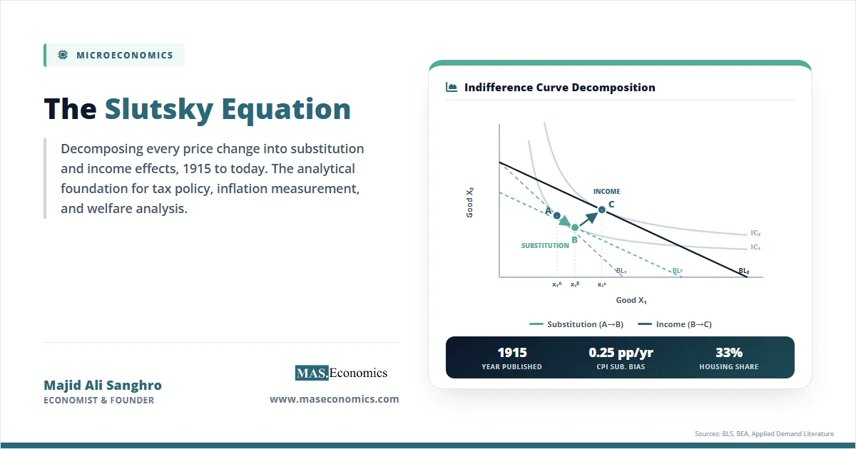
The same logic underlies the modern decomposition of price changes. When the price of good 1 changes, the consumer’s optimum shifts, and the change in chosen quantity can be split into a substitution effect and an income effect. The formal mathematics of that decomposition is the Slutsky equation, which uses the tangency condition as its starting point. The MRS is what makes the tangency condition meaningful, and the Slutsky equation is what unpacks the consumer’s response when prices move and the tangency point shifts.

When Indifference Curves Are Not Smooth

The clean derivative-based definition of MRS assumes the utility function is differentiable. Two important cases break this assumption, and seeing where they break clarifies what the standard assumption buys.

The first case is a perfect substitute. If the consumer regards two goods as functionally identical, say one-dollar bills and four quarters, the utility function is linear: \( u(x_1, x_2) = a x_1 + b x_2 \). Indifference curves are straight lines with slope \( -a/b \), and the MRS is the constant \( a/b \). Diminishing MRS fails because the willingness to substitute does not change with the bundle composition. At the optimum, the consumer typically chooses a corner solution, spending the entire budget on whichever good has the lower per-utility price.

The second case is a perfect complement. If the consumer needs goods in fixed proportions, say left shoes and right shoes, the utility function is \( u(x_1, x_2) = \min(a x_1, b x_2) \). Indifference curves are L-shaped, with a kink at the point where \( a x_1 = b x_2 \). The MRS is not defined at the kink, is zero along the horizontal segment, and is infinite along the vertical segment. The consumer’s optimum sits at the kink, where the budget line meets the corner of the L. No tangency condition applies because the indifference curve has no well-defined tangent at the kink.

These polar cases bracket the standard smooth-and-convex case in which the MRS is well-defined everywhere, varies continuously with the bundle, and falls as good 1 substitutes for good 2. Most empirical work assumes the smooth case, because it permits demand estimation through differentiable demand functions. The technical conditions that justify this assumption are exactly those laid out in the foundations of consumer preferences: monotonicity ensures the gradient of utility is positive, convexity ensures interior solutions, and differentiability ensures the MRS exists and varies smoothly. The Cobb-Douglas utility function \( u(x_1, x_2) = x_1^\alpha x_2^{1-\alpha} \) is the workhorse smooth case, with \( MRS = \frac{\alpha}{1-\alpha} \cdot \frac{x_2}{x_1} \), and it shows the typical pattern: the MRS depends on the bundle through the ratio \( x_2 / x_1 \) and falls as \( x_1 \) rises.

Reading the MRS in Real Consumption Data

The MRS is a theoretical construct, but it leaves observable footprints. Empirical demand systems recover marginal rates of substitution from the relationship between expenditure shares and relative prices in survey data. The Almost Ideal Demand System, developed by Angus Deaton and John Muellbauer in 1980 estimates a flexible functional form for the expenditure function and recovers MRS values for major consumption categories from observed budget shares.

The pattern in the data matches the theory. For food versus housing, the estimated MRS at typical household consumption levels is small for households spending a large share on housing and larger for households spending little on housing, consistent with diminishing MRS as housing consumption rises. For coffee versus tea specifically, the U.S. Consumer Expenditure Survey shows that coffee-heavy households have a higher MRS of tea for coffee than tea-heavy households, again consistent with the variety-preference interpretation. Cross-country comparisons show the same regularities, with the MRS between staples and luxuries varying systematically with income levels in ways that the Engel curve literature documents.

The MRS also plays a role in welfare measurement. When evaluating the effect of a tax or subsidy, the welfare loss to a consumer depends on the gap between the marginal social value of the taxed good and its marginal private value, which is mediated by the MRS at the consumer’s optimum. The deadweight loss formulas in public economics, including the Harberger triangle and its refinements, are derived using indifference-curve geometry where the MRS is the slope at the relevant tangency. The same logic carries into the response of demand to price changes through the structure of revealed preference, where the Weak Axiom of Revealed Preference implies the negativity of the substitution matrix, which in turn implies convex preferences and a well-behaved MRS.

From a Local Slope to a Theory of Choice

The marginal rate of substitution is a small idea with a large reach. It is local: it describes the slope at a single bundle. It is ordinal: it depends only on the ranking of bundles, not on cardinal utility levels. It is empirically grounded: it can be recovered from observed expenditure data with sufficient assumptions. And it is the hinge on which the consumer’s optimisation problem turns: the tangency between the indifference curve and the budget line is what selects the optimal bundle from the infinite set of affordable alternatives.

Diminishing MRS, the curvature property that makes the tangency unique and the optimum well-behaved, is the geometric statement of variety preference. It encodes the observation that consumers value balance, and it delivers the smooth, differentiable demand functions that empirical work depends on. When economists move from indifference curves to production isoquants, from consumer choice to producer choice, the same machinery reappears as the marginal rate of technical substitution, with the same diminishing property delivering the same well-posed optimisation problems. The MRS is, in this sense, the prototype of every marginal-trade-off concept in price theory.

Conclusion

The marginal rate of substitution is the slope of the indifference curve at a point, equal to the ratio of marginal utilities, and is the geometric core of consumer choice. It measures how much of one good a consumer will give up for one more unit of another while remaining indifferent. Diminishing MRS reflects variety preference and is equivalent to convex preferences. At the consumer’s optimum, the MRS equals the price ratio, which is the tangency condition that selects the utility-maximising bundle from the budget set. The concept extends to any number of goods, generalises to producer theory as the marginal rate of technical substitution, and provides the geometric foundation on which empirical demand systems and welfare measurement are built.

Frequently Asked Questions

Thanks for reading! If you found this helpful, share it with friends and spread the knowledge. Happy learning with MASEconomics