Excess Demand Function: Market Pressure

A market can face a shortage at one price and a surplus at another, but general equilibrium asks a harder question: whether all markets can clear at the same price vector. The excess demand function measures that pressure by showing how much buyers want to purchase beyond what sellers want to supply at each set of prices.

The function is not just a demand curve with another name. It is a net demand object. It combines planned demand, planned supply, endowments, budgets, and prices into one expression that tells whether a market is pushing prices upward, downward, or not at all.

In general equilibrium, excess demand functions connect all markets through the price vector. A change in one price can affect demand and supply in many other markets, so market pressure must be studied as a system.

Net demand drives adjustment

An excess demand function measures the gap between planned demand and planned supply at a given price. For a single good, the basic form is:

Single-Market Form

Positive excess demand means a shortage; negative excess demand means a surplus.

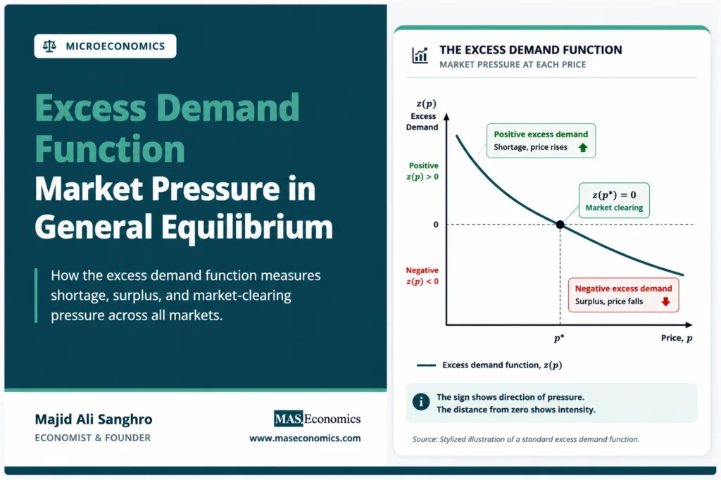
If \(z(p) > 0\), planned purchases exceed planned sales. Buyers want more of the good than sellers are willing to provide at that price. This creates upward price pressure. If \(z(p) < 0\), planned sales exceed planned purchases. Sellers are offering more than buyers want to buy, so price pressure is downward.

The market-clearing price is the price at which excess demand equals zero:

Market-Clearing Condition

At \(p^*\), the market is neither short nor long. Planned demand equals planned supply. The price does not have to move because the imbalance that would push it has disappeared.

This net-demand view is central because markets rarely need only demand or only supply. The pressure on price comes from their difference. A high demand curve matters for price only in relation to available supply, and a large supply schedule matters only in relation to planned demand.

The function maps prices to pressure

The word “function” matters. An excess demand function is not a single imbalance number. It maps each possible price into a corresponding level of excess demand.

At a low price, demand is usually high and supply is usually low, so excess demand tends to be positive. At a high price, demand is usually lower and supply is usually higher, so excess demand tends to be negative. The crossing point marks market clearing.

The diagram shows the central mechanism. Prices below \(p^*\) create positive excess demand. Buyers want more than sellers offer, so the market sends an upward pressure signal. Prices above \(p^*\) create negative excess demand. Sellers offer more than buyers want, so the market sends a downward pressure signal.

The curve does not have to be a straight line. Its shape depends on preferences, endowments, technologies, and substitution across goods. The important point is that the sign of \(z(p)\) tells the direction of pressure, while the distance from zero tells the size of the imbalance.

General equilibrium uses vectors

In general equilibrium, there is not one price and one excess demand function. There is a price vector and an excess demand vector. If an economy has \(n\) goods, the price vector is:

The excess demand function for good \(i\) depends on the entire price vector, not only on its own price:

General Equilibrium Form

Planned demand \(x_i(p)\) minus planned supply or endowment \(y_i(p)\), evaluated at the full price vector.

The full excess demand system is:

This vector form is the reason general equilibrium differs from ordinary single-market analysis. The excess demand for bread may depend on the wage, the price of grain, the price of substitutes, and household wealth. The excess demand for labor may depend on goods prices and firm production plans. The markets are linked through budgets and relative prices.

A general equilibrium price vector \(p^*\) clears all markets at once:

Equilibrium Price Vector

Here, zero means the zero vector. Every market included in the model has no excess demand. The condition is stronger than saying one market clears in isolation. It says all planned purchases and sales are mutually compatible at the same set of prices.

Walras law restricts the system

Excess demand functions are not arbitrary. In a complete general equilibrium model with budget constraints, they must satisfy Walras law:

Walras Law

The total value of excess demand across all markets equals zero.

This condition says that aggregate excess demand cannot have positive value across the whole economy. If buyers want more of some goods than sellers offer, they must want less of other goods, or they must be offering other assets, labor, or claims in exchange. The imbalance in one place must be matched by an offset elsewhere.

Walras law has a practical modeling implication. If all but one market clear, the remaining market must also clear, as long as its price is positive. This is why one market-clearing equation is often redundant in a general equilibrium system.

The economic meaning is straightforward. Excess demand is constrained by budgets. A household, firm, or trader can want a different bundle, but the value of desired purchases must be financed by the value of desired sales, income, or endowments. The excess demand function carries that accounting discipline into the market system.

Relative prices shape excess demand

Most general equilibrium models assume that excess demand functions are homogeneous of degree zero in prices. This means that if all prices are multiplied by the same positive number, excess demand does not change:

Homogeneity of Degree Zero

The reason is that only relative prices matter. If every price doubles, the budget set measured in real terms is unchanged. A good that cost twice as much now is bought with income or endowments that are also valued at twice as much. The money scale changes, but the real trade-offs do not.

This property explains the use of a numeraire. One price can be set equal to 1, and all other prices can be measured relative to it. The economy still has the same real allocation problem because the excess demand function responds to price ratios, not to the absolute units in which prices are written.

This same logic appears in Edgeworth Box analysis. The slope of the budget line matters because it reflects a relative price. Changing every price by the same proportion leaves the slope unchanged and therefore leaves the real exchange opportunities unchanged.

Price pressure guides adjustment

An excess demand function becomes dynamic when it is linked to a price-adjustment rule. A simple version says that price rises when excess demand is positive and falls when excess demand is negative:

Price-Pressure Rule

The price of good \(i\) moves in the direction of excess demand.

This is the logic behind the tatonnement process. Prices are adjusted in response to announced excess demands, and the system searches for a price vector where all excess demands disappear.

The excess demand function therefore plays two roles. It describes disequilibrium at a given price vector, and it provides the signal that a price-adjustment mechanism may use. A positive value says the price is too low relative to current plans. A negative value says the price is too high relative to current plans.

This does not prove that prices will converge. It only gives a direction of adjustment. In a many-market economy, raising one price can reduce excess demand in that market while changing excess demand elsewhere. Stability depends on how the entire vector \(z(p)\) behaves, not only on the sign of one component.

Individual plans aggregate into pressure

An aggregate excess demand function is built from individual plans. In a pure exchange economy, each agent begins with an endowment and chooses a preferred bundle subject to a budget constraint. The excess demand of agent \(h\) is the chosen bundle minus the initial endowment:

The aggregate excess demand function adds those individual excess demands:

Aggregation

This equation shows that excess demand is not a psychological measure of desire. It is a budget-constrained plan. Each agent’s desired net trade is limited by the value of that agent’s endowment. When those plans are added together, the market system reveals whether the current price vector makes all desired trades compatible.

If aggregate excess demand for a good is positive, the economy is collectively trying to acquire more of that good than is available at the current price. If aggregate excess demand is negative, the economy is collectively trying to dispose of more of that good than others want to hold. Market pressure is the aggregate result of many budget-constrained choices.

Properties limit possible shapes

Standard excess demand functions often satisfy several properties under familiar assumptions. They are usually continuous when preferences and technologies behave smoothly. They are homogeneous of degree zero when only relative prices matter. They satisfy Walras law when all markets and budget constraints are included.

These properties make the function usable in equilibrium analysis. Continuity helps formal existence arguments because small price changes do not create sudden jumps in excess demand. Homogeneity permits price normalization. Walras law links the market equations together and prevents the model from creating net purchasing power.

Table 1. Core properties of excess demand functions

Property	Formal idea	Economic meaning
Market clearing	\(z_i(p^*) = 0\)	Planned demand equals planned supply.
Walras law	\(p \cdot z(p)=0\)	Excess demands balance in value.
Homogeneity	\(z(\lambda p)=z(p)\)	Only relative prices matter.
Continuity	Small price changes imply small demand changes.	Equilibrium analysis becomes mathematically tractable.
Central role	\(z(p)\) summarizes market pressure.	It links individual plans to system-wide clearing.
Source: MASEconomics editorial synthesis based on standard general equilibrium theory.

The properties are useful, but they do not make the function simple. A general excess demand function can behave in complicated ways once many agents, many goods, and cross-market substitutions are included. The system may have more than one equilibrium, or price adjustment may fail to settle on a stable point.

Partial equilibrium misses feedback

In partial equilibrium, excess demand can be studied in one market while other prices are held constant. This is useful for many practical questions, especially when one market is small relative to the rest of the economy. A single excess demand curve can show the pressure on the price of one good.

General equilibrium changes the problem. The excess demand for one good may depend on the prices of many other goods. A rise in the price of energy can affect labor demand, goods prices, transport costs, and household consumption plans. The excess demand function becomes part of a connected system rather than a stand-alone curve.

This is why excess demand functions matter beyond ordinary supply and demand. A single market diagram can show shortage and surplus. A general equilibrium excess demand system shows how shortages and surpluses across markets fit together under budget constraints.

The distinction is not a rejection of partial equilibrium. It is a boundary around its use. When feedback from other markets is small, partial equilibrium is often enough. When feedback is central, the excess demand function must be studied as part of the full price vector.

Explains

Conclusion

Excess demand function analysis shows how prices translate individual plans into market pressure. A positive value signals shortage and upward price pressure; a negative value signals surplus and downward price pressure; a zero value signals market clearing.

In general equilibrium, the function becomes a vector that links all markets through relative prices and budget constraints. It must respect Walras law, it usually depends on price ratios rather than absolute price levels, and it provides the signal used in price-adjustment processes such as tatonnement.

The concept is powerful because it connects disequilibrium to equilibrium without assuming that markets automatically clear. It identifies where pressure exists, how that pressure is measured, and why clearing one market cannot be separated from the rest of the economic system.

Frequently Asked Questions

Thanks for reading! If you found this helpful, share it with friends and spread the knowledge. Happy learning with MASEconomics