Generalized Method of Moments: Unified Estimation Framework

Robert Hall’s 1978 test of the consumption Euler equation revealed that consumption growth is unforecastable, but it also exposed a methodological gap: the Euler equation is a conditional expectation, not a regression. The generalized method of moments, formalized by Lars Peter Hansen in his 1982 Econometrica paper, was the estimation framework built precisely for this kind of problem, and it earned Hansen the 2013 Nobel Prize in Economics.

GMM is not a single estimator. It is a unifying principle. Almost every classical estimator in econometrics, including OLS, instrumental variables, two-stage least squares, and maximum likelihood under the right setup, can be derived as a special case of GMM. The framework asks the researcher to write down a set of moment conditions that the data must satisfy if the model is true, and then chooses the parameters that make those moment conditions hold as closely as possible in the sample. The generality is what makes the method powerful, and the moment conditions are what give each application its economic content.

Defining the Moment Condition

A moment condition is a statement of the form: at the true value of the parameter, the expected value of some function of the data is zero. The function is chosen so that the statement is implied by the economic model.

Population Moment Condition

z_t is the data at observation t, θ_0 is the true parameter vector, and g(·) is a function whose population expectation is zero when evaluated at the true parameter.

The economic content of the model lives entirely inside the function g. In an ordinary linear regression with no endogeneity, the moment condition is that the regressors are uncorrelated with the error term: \(E[x_t(y_t – x_t’ \theta)] = 0\). In an instrumental variables setting, the moment condition is that the instruments are uncorrelated with the structural error: \(E[z_t(y_t – x_t’ \theta)] = 0\), where z_t is the instrument vector. In the consumption Euler equation, the moment condition is that the deviation between the realized marginal-utility-weighted return and one, multiplied by any variable in the agent’s information set, has expectation zero.

The same logical structure runs through every application. The model says something must be true on average. The sample analog of that statement is the average of \(g(z_t, \hat{\theta})\) across observations. The GMM estimator chooses \(\hat{\theta}\) to make that sample average as close to zero as possible.

Sample Analog and Identification

The population moment condition cannot be evaluated directly, because the population is not observed. The researcher works with the sample analog:

Sample Moment Condition

T is the sample size. The sample moment converges in probability to the population moment as T grows.

When the model has k parameters and exactly k moment conditions, the system is exactly identified. There is a unique parameter vector that sets \(\bar{g}_T(\theta) = 0\), and GMM reduces to solving that system. This is the case that classical method-of-moments estimation handles, and it covers many simple examples including OLS.

The harder and more interesting case arises when the number of moment conditions exceeds the number of parameters. The system has more equations than unknowns, and in general no single parameter vector can satisfy all the moment conditions simultaneously. This is the overidentified case, and it is exactly the situation that arises in the Euler equation example. If consumption growth is uncorrelated with current information, then it is uncorrelated with last period’s consumption growth, with last period’s interest rate, with last period’s income, and with any other lagged variable. Each of these gives a separate moment condition, but the consumption Euler equation has only a handful of parameters to estimate. The system is overidentified, and the resolution is to find the parameter vector that comes closest to satisfying all the moment conditions in a weighted sense.

GMM Criterion Function

Hansen’s formal solution to the overidentification problem is to minimize a quadratic form in the sample moment conditions, with a weighting matrix that determines how much each moment condition matters in the overall fit.

GMM Estimator

W is a positive-definite weighting matrix that determines how the moment conditions are aggregated into a single objective function.

The criterion function is a weighted sum of squared moment deviations. If W is the identity matrix, every moment condition gets equal weight. If W is the inverse of the covariance matrix of the sample moments, the moment conditions that are more precisely estimated get more weight, and the estimator achieves the smallest possible asymptotic variance within the class of GMM estimators. This second choice, the efficient weighting matrix, is the result that gives Hansen’s paper its theoretical depth.

The efficient choice cannot be implemented in one step, because the covariance matrix of the moments depends on the unknown parameter. The standard solution is a two-step procedure. The first step uses a simple weighting matrix, often the identity, to obtain an initial consistent estimate of \(\theta\). The residuals from this first step are used to estimate the covariance matrix of the moments, which is then inverted to give the optimal weighting matrix. The second step minimizes the criterion function using this optimal weighting matrix, producing the efficient GMM estimator.

A common refinement iterates this procedure until convergence, updating the weighting matrix and the parameter estimate simultaneously. The iterated GMM estimator coincides with continuous-updating GMM in many cases and has better finite-sample properties than the standard two-step estimator. In small samples, the choice between two-step, iterated, and continuous-updating versions can matter; in large samples, all three converge to the same asymptotic distribution.

Euler Equation Estimation

The consumption Euler equation comes from a standard household problem. A representative agent chooses consumption \(c_t\) to maximize the expected present value of utility, subject to a budget constraint. The first-order condition for intertemporal optimization is:

Euler Equation

β is the discount factor, u'(·) is marginal utility, r_{t+1} is the asset return between t and t+1, and ℐ_t is the agent’s information set at time t.

For an isoelastic utility function with coefficient of relative risk aversion \(\gamma\), the marginal utility ratio simplifies to \((c_{t+1}/c_t)^{-\gamma}\), and the Euler equation becomes a tractable expression in observable consumption growth and asset returns. Rewriting the conditional moment condition in unconditional form by multiplying both sides by any variable in the agent’s information set produces a set of moment conditions that can be taken to the data. The economic structure behind this consumption decision is treated more carefully in the article on the permanent income hypothesis, and the Euler-equation logic also underpins the household side of the Ramsey growth model.

The moment conditions take the form:

Operational Moment Conditions

z_t is any vector of variables in the agent’s information set, typically lagged consumption growth, lagged returns, lagged income growth, and a constant.

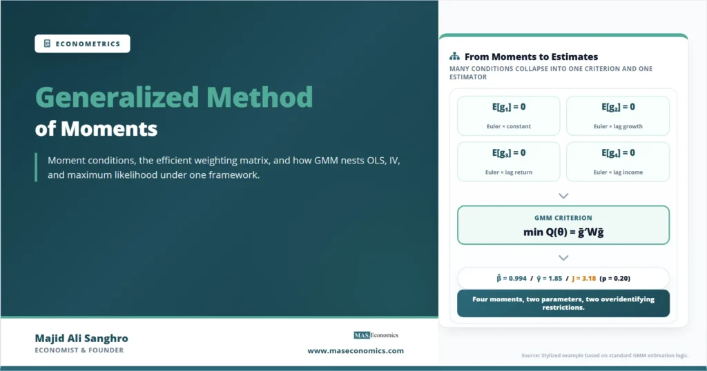
If z_t has, say, four elements, the system has four moment conditions and only two parameters (the discount factor \(\beta\) and the risk aversion \(\gamma\)). The system is overidentified, and the GMM estimator chooses \(\hat{\beta}\) and \(\hat{\gamma}\) to minimize the weighted quadratic form in the sample moments. The output of this exercise on a typical postwar US quarterly dataset looks roughly as follows.

Table 1. GMM Estimates of the Consumption Euler Equation

Parameter	Two-step GMM	Iterated GMM	Economic interpretation
Discount factor β	0.994***	0.992***	Quarterly time preference rate ~0.7%
Risk aversion γ	1.85***	2.04***	Low to moderate by standard estimates
Standard error (β)	(0.003)	(0.003)	Precise estimate of discount factor
Standard error (γ)	(0.42)	(0.48)	Moderate uncertainty in risk aversion
Moment conditions	4	4	Constant + 3 lagged instruments
Parameters	2	2	β and γ
Overidentifying restrictions	2	2	Tested via the J statistic
Hansen J statistic	3.18	2.94	p = 0.20 / 0.23, cannot reject moments
Source: Stylized example based on standard consumption-Euler GMM formulas. Significance: *** p < 0.01.

The estimated discount factor of around 0.99 implies a quarterly time-preference rate of roughly 0.7 percent, or about 2.8 percent annualized. The estimated risk aversion of around 1.9 to 2.0 is on the low end of what calibration exercises in macroeconomics typically assume, which is part of why empirical Euler equation studies have generated long-running debates about the equity premium and other puzzles. The Hansen J statistic of around 3 against a chi-squared distribution with two degrees of freedom gives a p-value above 0.20, so the overidentifying restrictions are not rejected. The model is statistically consistent with the data, even though the estimated parameters look small relative to what asset-pricing applications often require.

The Logic of the J Test

The Hansen J statistic is a direct byproduct of the GMM estimation procedure. After the efficient weighting matrix has been computed and the parameters estimated, the value of the criterion function at the optimum can be evaluated against a chi-squared distribution to test the overidentifying restrictions.

Hansen J Statistic

T is the sample size, q is the number of moment conditions, k is the number of parameters, and the degrees of freedom equal the number of overidentifying restrictions q – k.

If the model is correctly specified, all the moment conditions hold in the population, and the J statistic converges to a chi-squared distribution with q minus k degrees of freedom. A small J statistic and a large p-value mean the overidentifying restrictions are consistent with the data. The model is not rejected, and the additional moment conditions beyond those needed for identification appear to be implied by the same parameter values that satisfy the just-identified subset.

A large J statistic is more informative than it might first appear. It says the parameter vector that best satisfies one subset of moment conditions cannot also satisfy the others. The model is statistically inconsistent with the data, and the standard interpretation is that the model is misspecified in some way. The J test does not point to which moment condition is violated, only that the joint system fails. Diagnosing which moment is the source of the rejection requires further specification analysis.

GMM Generalizes Classical Estimators

GMM is not just one more estimator in the toolbox. It is the framework that contains most of the others as special cases, and the reduction in each case is straightforward.

OLS is the GMM estimator for the moment condition \(E[x_t(y_t – x_t’ \theta)] = 0\) with the identity weighting matrix. The system is exactly identified, the criterion function has a closed-form minimum, and the resulting estimator is the ordinary least squares formula. This is the cleanest illustration of how the GMM principle nests classical regression.

Two-stage least squares and the broader instrumental variables estimator are GMM applied to the moment condition \(E[z_t(y_t – x_t’ \theta)] = 0\), where z_t is the instrument vector. When the system is exactly identified, with the number of instruments equal to the number of endogenous regressors, GMM and IV coincide. When the system is overidentified, GMM with the efficient weighting matrix delivers the most efficient combination of the moment conditions, which is what two-stage least squares achieves under homoskedasticity. With heteroskedasticity, GMM with a heteroskedasticity-robust weighting matrix is strictly more efficient than two-stage least squares, which is one of the main reasons GMM became the default in cross-sectional applied work after the 1990s.

Maximum likelihood estimation is GMM applied to the score function of the log-likelihood. The score is the gradient of the log-likelihood with respect to the parameters, and its expectation is zero at the true parameter under standard regularity conditions. Treating this as a moment condition and applying GMM with the inverse Fisher information as the weighting matrix delivers the maximum likelihood estimator with the standard asymptotic variance. The relationship between GMM and likelihood-based estimation is explored further in the article on maximum likelihood estimation.

The fact that all of these estimators are special cases of GMM is not just a theoretical curiosity. It means that the same standard-error formulas, the same robust-variance corrections, and the same specification tests can be applied uniformly. A researcher who understands GMM thoroughly has a single inferential framework that covers most of what applied econometrics needs, with the moment conditions changing from application to application but the underlying logic remaining the same.

Weighting Matrix Role

The choice of weighting matrix is what separates GMM from classical method-of-moments estimation. In the just-identified case it does not matter, because the moment conditions can all be set to zero exactly. In the overidentified case, the weighting matrix determines how much each moment condition matters for the parameter estimate.

The efficient choice is the inverse of the covariance matrix of the moments, often called the optimal weighting matrix. This choice gives the smallest possible asymptotic variance among the class of GMM estimators that use the same moment conditions. The efficiency gain comes from down-weighting moments that are imprecisely estimated and up-weighting moments that are tightly identified.

In practice, the optimal weighting matrix is estimated from the data, and its finite-sample properties can be problematic when the number of moment conditions is large relative to the sample size. With many moments and a modest sample, the estimated weighting matrix can be unstable, and the resulting GMM estimator can be biased and have poor coverage properties. The empirical literature on weak instruments and many-instrument bias developed largely in response to this problem, and modern practice often involves choosing a smaller, more carefully justified set of moment conditions rather than throwing every available lag into the system.

An alternative that has gained traction is continuous-updating GMM, in which the weighting matrix is treated as a function of the parameter and is updated simultaneously with the parameter estimate within a single optimization problem. Continuous-updating GMM tends to have better small-sample properties than the two-step estimator, particularly in weak-identification settings, at the cost of being computationally more demanding.

GMM in Applied Economics

The reach of the GMM framework into applied economics is broader than any single application can convey. Three areas illustrate the pattern.

In asset pricing, GMM is the standard tool for estimating consumption-based and factor-based pricing models. The moment conditions come directly from the no-arbitrage and intertemporal optimization conditions of the model, and the data are returns on different portfolios. The equity premium puzzle, the equity term structure puzzle, and the broader literature on stochastic discount factors all rest on GMM estimation of moment conditions implied by asset-pricing theory. The strength of GMM in this setting is that the moment conditions are direct implications of the theoretical model, and rejection of the overidentifying restrictions is informative about whether the theory is consistent with the data.

In labor and household economics, GMM is used to estimate dynamic discrete-choice models, life-cycle consumption-saving models, and search models with heterogeneous agents. The moment conditions in these applications often combine first-order conditions from the agent’s optimization problem with empirical moments drawn from cross-sectional and longitudinal data. The household-saving framework that motivates many of these models, including the role of consumption smoothing across the life cycle, is treated in the article on the consumption function.

In macroeconomics, GMM is the workhorse estimator for the structural parameters of dynamic stochastic general equilibrium models when full-information likelihood methods are impractical. The moment conditions are derived from the linearized first-order conditions of the model, often supplemented by reduced-form moments from impulse responses or unconditional second moments. The flexibility of the GMM framework allows researchers to focus identification on the parameters that are most economically interesting while leaving other features of the model less tightly constrained.

Limits of the Framework

GMM is powerful, but it is not a free lunch, and the conditions for it to work well deserve more attention than they usually receive.

The first limit is weak identification. If the moment conditions are not informative about the parameters, the GMM estimator can be severely biased, and standard inference can be deeply misleading. The weak-instrument problem in IV is a special case of this broader concern, and the same logic applies to any GMM application where the moments are nearly flat with respect to the parameters. Diagnostic tests for weak identification have become a standard part of careful GMM practice in the modern literature.

The second limit is the validity of the moment conditions. The framework assumes the population moments equal zero at the true parameter. If this assumption is wrong, the GMM estimator converges to whatever value of the parameter best satisfies the wrong moments, and this value generally has no economic interpretation. The J test detects gross misspecification, but a passing J test does not prove the moment conditions are correct. It only fails to reject them.

The third limit is finite-sample performance. The asymptotic theory underlying GMM standard errors and test statistics relies on large samples, and small-sample distributions can depart substantially from their asymptotic counterparts. With many moment conditions, with persistent data, or with weak instruments, the gap between asymptotic and finite-sample performance can be large enough to invalidate routine inference. Bootstrap methods and small-sample corrections have been developed to address these issues, but their use remains uneven in applied practice.

The fourth limit is interpretive. GMM gives consistent estimates of the parameters that satisfy a particular set of moment conditions. It does not, by itself, identify the structural model that generated the data. A model with different structural parameters can produce the same moment conditions, and GMM cannot distinguish between them. This is the standard identification problem that runs through all of structural econometrics, and GMM provides a powerful estimation method given a successful identification argument rather than a substitute for one.

Explains

Conclusion

The generalized method of moments turned a scattered collection of econometric techniques into a single framework. By starting from moment conditions implied by the economic model and minimizing a weighted quadratic form in the sample moments, GMM produces estimators that nest OLS, instrumental variables, two-stage least squares, and maximum likelihood under their respective moment conditions. The overidentified case, in which more moment conditions exist than parameters, is where the framework earns its place: it allows researchers to combine multiple implications of a theory into a single estimator and to test whether all the implications are jointly consistent with the data through the Hansen J statistic.

The framework’s strength is its flexibility. The economic content of any application lives entirely inside the moment conditions, and the same estimation machinery applies regardless of whether the moments come from a consumption Euler equation, an asset-pricing model, a dynamic discrete-choice model, or a linearized DSGE system. The framework’s weakness is the same as its strength. Weak moment conditions, misspecified moment conditions, and finite-sample departures from asymptotic theory can all undermine the estimator, and a careful applied researcher pays attention to all three when interpreting GMM results.

The continuing influence of GMM on empirical economics reflects the importance of the underlying insight. Most economic models do not deliver clean regression equations. They deliver conditional expectations, orthogonality conditions, and first-order conditions that any reasonable estimator must respect. Hansen’s 1982 framework was the first general procedure for taking these statements directly to the data, and three decades later it remains the standard tool for doing so. The connection between GMM and the broader project of estimating structural economic relationships, from multiple regression models through dynamic equilibrium systems, runs through every modern econometrics curriculum and through a large share of the empirical literature in macroeconomics, finance, and applied microeconomics.

Frequently Asked Questions

Thanks for reading! If you found this helpful, share it with friends and spread the knowledge. Happy learning with MASEconomics