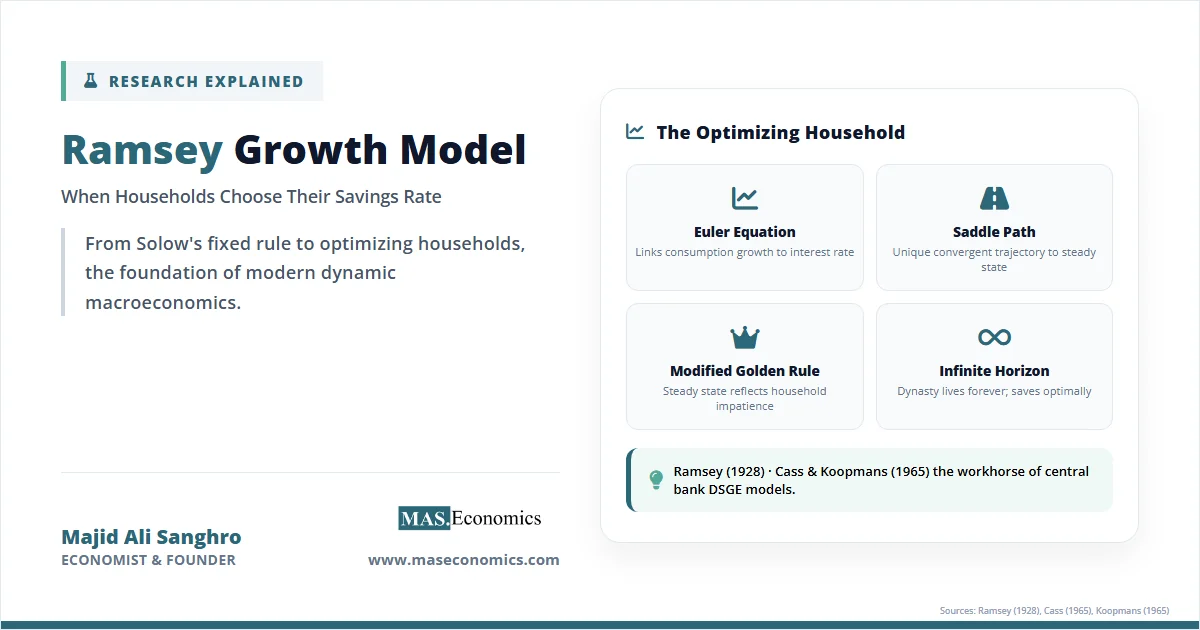
The Ramsey growth model economics framework solved a problem that haunted Robert Solow’s celebrated 1956 growth model: where does the savings rate come from? Solow simply assumed it. Households in his world saved a constant fraction of income, year after year, regardless of interest rates, life-cycle position, or expectations about the future. The Ramsey-Cass-Koopmans (RCK) model rewrote that assumption from the ground up. Households choose their savings rate by maximizing lifetime utility, weighing consumption today against consumption tomorrow.
This shift mattered far beyond growth theory. By 1928, when Frank Ramsey published the original mathematical version, he was solving a normative question. By 1965, when David Cass and Tjalling Koopmans extended it independently, the model had become the workhorse of dynamic macroeconomics. Today every major dynamic stochastic general equilibrium (DSGE) model used by the Federal Reserve, the European Central Bank, and the IMF rests on Ramsey’s foundation: an optimizing household, an Euler equation, and a transversality condition.
The RCK model also produces sharper policy implications than Solow’s. Because savings respond to incentives, tax cuts on capital, government spending shocks, and monetary policy interventions all change the path of consumption and investment in ways that depend on household preferences. Understanding the model means understanding the language modern central banks speak.
The Logic of Ramsey’s Household
The core idea of the Ramsey growth model is that an infinitely-lived representative household chooses a consumption path that maximizes the discounted sum of lifetime utility, subject to a capital accumulation constraint. The household is forward-looking and rational. It values consumption today more than consumption tomorrow, but it also recognizes that saving means more capital, more output, and more consumption later.
Ramsey originally framed the problem from the perspective of a benevolent social planner. The planner chooses how much output to consume and how much to invest in capital so as to maximize society’s welfare. Cass and Koopmans showed in 1965 that this planner’s solution coincides with the outcome of a decentralized competitive equilibrium, where firms hire capital and labor at market prices and households trade in perfect financial markets. With no market imperfections, the first welfare theorem holds, and the two solutions are identical. This equivalence is one reason the model became so influential.
At the heart of the model is the Euler equation. This first-order condition tells us how consumption must grow over time if the household is behaving optimally. The intuition is simple. If the marginal product of capital exceeds the household’s rate of time preference, households want to save more, accumulate capital, and increase consumption later. If the marginal product falls below the rate of time preference, households want to consume more today and run capital down. Optimal behavior balances these two forces. Solow’s fixed savings rate had no such mechanism. Households in Ramsey’s world adjust their savings rate continuously in response to the marginal product of capital, the real interest rate, and their preferences.
The model also produces a unique steady state, called the modified golden rule. Unlike Solow’s golden rule (which maximizes steady-state consumption mechanically), the modified golden rule reflects household impatience. The steady-state capital stock is lower than Solow’s golden-rule level because households discount future utility. They are not willing to sacrifice consumption today to reach the maximum-consumption steady state if it takes too long to get there.
Ramsey Model in Equations
The household maximizes the present discounted value of utility from per-capita consumption \( c(t) \) over an infinite horizon:
where \( \rho \) is the rate of time preference. The capital stock per worker evolves according to the law of motion:
Here \( f(k) \) is output per worker (a neoclassical production function such as Cobb-Douglas), \( n \) is the population growth rate, and \( \delta \) is the depreciation rate of capital. The household takes the path of wages and interest rates as given in the decentralized version, or the planner internalizes them in the centralized version.
To solve the problem, we use the Hamiltonian:
The first-order conditions yield the canonical Keynes-Ramsey rule (also called the consumption Euler equation). With a constant relative risk aversion (CRRA) utility function:
The Euler equation takes the form:
Consumption per capita grows when the net marginal product of capital, \( f'(k) – \delta \), exceeds the effective discount rate \( \rho + \theta n \). The parameter \( \theta \) is the inverse of the intertemporal elasticity of substitution. A high \( \theta \) means households dislike volatility in their consumption path and resist large changes even when interest rates move.
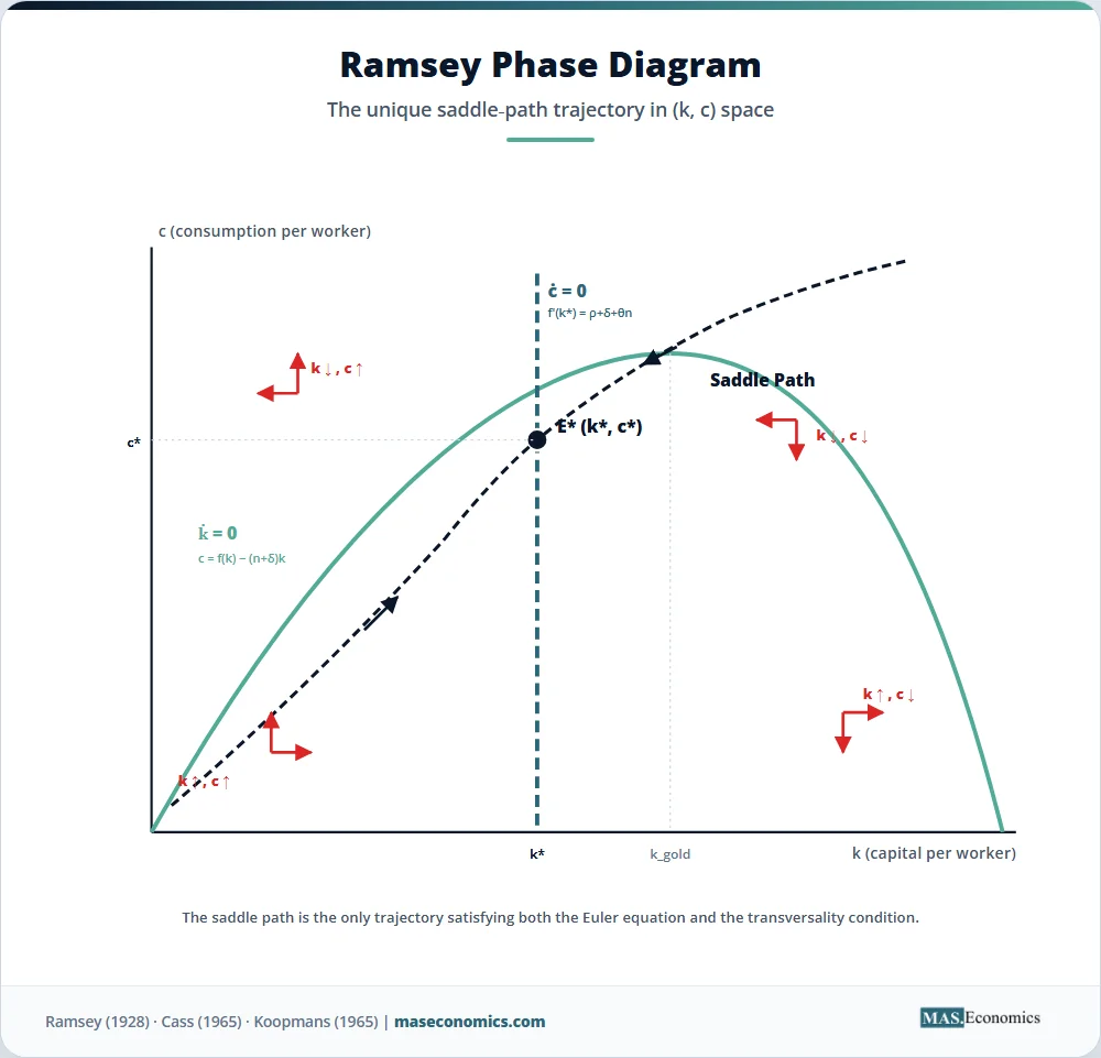
The phase diagram in \( (k, c) \) space has two key loci:
The \( \dot{k} = 0 \) locus, where investment exactly offsets depreciation and population growth. This is a hump-shaped curve in \( (k, c) \) space.
The \( \dot{c} = 0 \) locus, where consumption is constant. From the Euler equation, this requires \( f'(k^*) = \rho + \delta + \theta n \), which pins down the steady-state capital stock \( k^* \) as a vertical line.
The two loci intersect at the unique steady state \( (k^*, c^*) \). Around this point, the dynamics are saddle-path stable. There is exactly one trajectory, the saddle path, that converges to the steady state. Cass deduced a transversality condition from sections of a book by Pontryagin, which rules out paths leading to zero consumption or zero capital. This transversality condition is what makes the saddle-path solution unique.
| Symbol | Meaning | Typical Value |
|---|---|---|
| \( c(t) \) | Per-capita consumption at time \( t \) | Endogenous |
| \( k(t) \) | Per-worker capital stock | Endogenous |
| \( f(k) \) | Per-worker production function | Cobb-Douglas: \( k^{\alpha} \) |
| \( \rho \) | Rate of time preference | 0.02 to 0.04 per year |
| \( \theta \) | Coefficient of relative risk aversion | 1 to 4 |
| \( \delta \) | Capital depreciation rate | 0.05 to 0.10 per year |
| \( n \) | Population growth rate | 0.01 to 0.02 per year |
| \( \alpha \) | Capital share in output | 0.30 to 0.40 |
| \( \lambda(t) \) | Costate variable (shadow price of capital) | Endogenous |
 | ||
Table 1. Variable Glossary: Parameters and endogenous quantities in the Ramsey-Cass-Koopmans model.
One technical condition matters for the model to have a well-defined solution. Lifetime utility must be bounded, which requires \( \rho – n > (1-\theta) g \), where \( g \) is the growth rate of labor-augmenting technology. If this fails, the integral diverges, and the optimization problem has no solution.
Key Assumptions and Shortcomings
The Ramsey growth model rests on assumptions that are powerful but restrictive. The household lives forever. There is one representative household whose preferences capture the entire economy. Markets are complete and frictionless. Information is perfect, and households have rational expectations or perfect foresight. There are no externalities, no taxes that distort behavior, and no liquidity constraints.
The infinite horizon assumption is less innocent than it sounds. Infinite lives can be defended as a stand-in for households with operative bequest motives, where parents care about their children’s utility. In that interpretation, the dynasty lives forever even if individuals do not. But the assumption fails in overlapping generations (OLG) models, where finite lives create wealth transfers between cohorts. In OLG models, Ricardian equivalence does not hold. A bond-financed tax cut today raises consumption because the future taxes that pay back the debt fall on a generation not yet alive. The Ramsey model, by contrast, predicts that the household saves the entire tax cut to pay future taxes, leaving consumption unchanged.
The representative agent assumption hides distributional questions entirely. Two economies with identical aggregate consumption but very different inequality look the same in a Ramsey model. This was acceptable for early growth theory, but it is increasingly unacceptable today. Modern Heterogeneous Agent New Keynesian (HANK) models replace the representative household with a distribution of households facing idiosyncratic income risk and borrowing constraints. HANK models generate marginal propensities to consume that match the data far better than Ramsey models, and they show that monetary policy works through different channels for poor and rich households.
Habit formation is another important extension. Standard Ramsey utility depends only on current consumption, but real households appear to compare current consumption to past consumption. Habit-formation models, where utility depends on \( c_t – h c_{t-1} \), generate smoother consumption responses to shocks and help explain the equity premium puzzle.
How the Model Fits the Data
How well does the Ramsey model survive contact with data? The answer is mixed and revealing. The model’s most testable prediction is the Euler equation itself. Robert Hall’s 1978 paper introduced the random walk model of consumption, which derives directly from the Euler equation under the assumption of rational expectations and a quadratic utility function. Hall showed that if households optimize, then changes in consumption should be unpredictable using past information. Only news that arrives between periods should move consumption.
Using postwar aggregate US data, Hall found that past consumption data have no power in predicting future consumption. He could not reject the random-walk hypothesis with lagged income or lagged consumption as predictors. This was a striking confirmation. But subsequent research told a more complicated story. Many authors found that the orthogonality condition does not hold unconditionally in the data, and Flavin in 1981 challenged it with aggregate data. The phenomenon was called excess sensitivity: consumption responds too strongly to predictable changes in income, which the Euler equation rules out. Studies using household-level data have found similar puzzles.
The most famous failure is the equity premium puzzle, identified by Mehra and Prescott in 1985. The Ramsey-Lucas asset pricing model, a stochastic version of the RCK Euler equation, predicts that the equity premium should be small under reasonable risk aversion. Actual US data showed an equity premium of around 6 percentage points per year, which the standard model can only generate with implausibly high values of \( \theta \). This puzzle launched a vast literature on alternative preferences, including Epstein-Zin recursive utility and habit formation.
Calibration exercises tell a more positive story. When researchers feed plausible parameter values into a Ramsey model, they can generate consumption paths that broadly track aggregate data over long horizons. The model captures the key qualitative feature of consumption smoothing: households use saving and dis-saving to insulate consumption from income fluctuations. The chart below compares a simulated consumption path from a calibrated Ramsey model with US per-capita real consumption.
Figure 1. Simulated consumption from a calibrated Ramsey model versus US real per-capita consumption (indexed, 1980 = 100). Sources: Bureau of Economic Analysis; author’s simulation using \( \theta = 2 \), \( \rho = 0.03 \), \( \alpha = 0.35 \).
The simulated path matches the broad trend but misses the cyclical fluctuations, especially the 2008-2010 collapse. This is the model’s well-known weakness: it explains long-run growth and consumption smoothing, but it does not generate realistic business cycles without further extensions such as productivity shocks, sticky prices, or financial frictions. Modern DSGE models add these layers to the Ramsey core.
Ramsey’s Lasting Policy Influence
The Ramsey model is the bedrock of modern dynamic macroeconomics. Every Smets-Wouters-style DSGE model used by central banks today has a Ramsey household at its core. The Federal Reserve’s FRB/US model, the European Central Bank’s New Area-Wide Model (NAWM), and the IMF’s Global Integrated Monetary and Fiscal Model (GIMF) all rely on optimizing households whose behavior is governed by Euler equations. When the Fed staff presents a forecast to the FOMC, the underlying machinery is Ramsey’s machinery, layered with rigidities and shocks.
This matters because policy evaluation requires welfare metrics, and welfare metrics require optimizing households. The Solow model has no concept of welfare. It has output and capital, but no preferences. The Ramsey model has a utility function, which lets economists compute the welfare cost of inflation, the welfare gain from tax reform, or the welfare effect of fiscal stimulus. When the Congressional Budget Office estimates the long-run effect of a tax bill, the calculation typically rests on a Ramsey-style framework with optimizing households responding to changes in after-tax interest rates.
The model also clarifies the difference between transitory and permanent shocks. A temporary government spending increase produces a small response because households know it will end. A permanent increase produces a larger response. This distinction, which has no analog in a fixed-savings-rate Solow model, drives much of the policy analysis in modern macro. It also underpins the Ricardian equivalence proposition that bond-financed deficits do not stimulate consumption when households are forward-looking and infinite-lived.
For monetary policy, the Euler equation is the mechanism through which interest rates affect consumption. When the Fed cuts rates, the marginal product of capital falls, the Euler equation tilts the consumption path toward the present, and current consumption rises. The strength of this response depends on \( \theta \). With \( \theta = 1 \), the elasticity of consumption with respect to the real interest rate is one. With \( \theta = 4 \), it is one-quarter. Estimates of \( \theta \) from microeconomic studies suggest values between 1 and 2, which is one reason monetary policy transmission through the Euler-equation channel is often weaker in models than central bankers want.
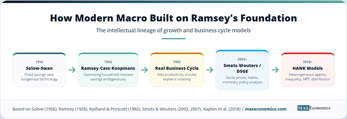
The Ramsey model also forms the bridge between the older Solow-Swan growth model and modern endogenous growth theory. Solow took the savings rate as given. Ramsey derived it from preferences. Romer and Lucas, in the 1980s, went further by deriving the rate of technological progress from optimizing decisions about R&D and human capital. Each step in this progression added another layer of micro-foundations. The connection to the consumption function is direct: the Euler equation is a forward-looking consumption function in which today’s consumption depends on expectations about all future income and interest rates. The permanent income hypothesis is a special case of the Ramsey model with quadratic utility, and dynamic programming provides the mathematical machinery for solving its stochastic extensions.
Practical applications appear across G7 economies. UK fiscal policy debates routinely invoke Ramsey-style logic when arguing about the long-run effects of debt accumulation. The Bank of Canada’s Terms-of-Trade Economic Model embeds a Ramsey household with habit formation. The Reserve Bank of Australia’s MARTIN model uses optimizing consumers to evaluate the long-run impact of immigration and productivity shocks. The model is not just a textbook artifact. It is the operational language of forecasting.
MASEconomics Explains
Four economic concepts behind the Ramsey growth model
Conclusion
The Ramsey growth model economics framework is the bedrock on which modern dynamic macroeconomics is built. By replacing Solow’s fixed savings rate with a forward-looking household that maximizes lifetime utility, Ramsey, Cass, and Koopmans created a model in which savings, capital accumulation, and consumption all emerge from preferences and prices. The Euler equation, the saddle path, and the modified golden rule are direct consequences of that optimization.
The model has empirical limitations. The equity premium puzzle, excess sensitivity of consumption to predictable income, and the failure of the representative-agent assumption to capture inequality all show where Ramsey’s framework falls short. Yet every modern central bank model and every welfare-based policy evaluation uses the Ramsey core, often layered with habits, sticky prices, and heterogeneous agents. Solow gave us the long-run capital stock. Ramsey gave us the household behind it.
Did you find this article helpful? Share it with someone who loves economics. And remember, at MASEconomics, we make complex ideas simple.