Heckman Selection Model: Correcting Sample Selection Bias

The Heckman selection model addresses a puzzle that standard regression could not solve in labor force surveys of the late 1960s. Researchers sought to estimate how women’s wages responded to education and experience, but wages were observed only for those who worked. The data excluded non-participants, whose potential wages were missing. Ordinary regression on workers alone produced biased estimates because women who chose to work had systematically better unobserved characteristics. The model formalized this selection problem and provided the two-stage correction that made the wage equation interpretable again.

The contribution was not only a statistical fix. Heckman showed that sample selection is a specific case of an omitted-variable problem, and that the omitted variable could be reconstructed from a model of the selection decision itself. The technique earned Heckman the 2000 Nobel Prize in Economics and reshaped a generation of empirical work in labor economics, development economics, education, and any setting where the outcome of interest is observed only for a non-random subset of the population.

Sample Selection in the Data

A regression coefficient is meaningful only when the data used to estimate it are representative of the population the researcher wants to describe. Sample selection breaks that representativeness. The breakdown is not a problem of small samples or measurement error; it is a problem of which observations enter the dataset in the first place.

Consider the wage equation in its classical form. Let \(w_i\) be the log wage of person i, and let \(z_i\) be a vector of characteristics, including education, experience, and demographic controls. The model the researcher would like to estimate is:

Wage Equation

η_i is the wage equation error term, capturing factors that affect log wages beyond the observed characteristics.

The estimation problem is that \(w_i\) is observed only for people who work. For people who do not work, the dataset contains z_i but not w_i. If the decision to work is itself driven by expected wages, then the people who appear in the wage data are systematically different from the people who do not. They are not a random sample; they are a selected sample. Running OLS on the workers alone estimates the conditional expectation of wages given that someone chose to work, which is generally not the same as the unconditional expectation that the wage equation is supposed to identify.

The intuition is concrete in the women’s labor supply case. Suppose two women have identical education and experience, but one woman has access to a higher-paying offer for reasons not captured in the data, such as a network connection or an unmeasured skill. She accepts the offer, and her wage appears in the data. The other woman receives a lower offer and remains out of the labor force. The dataset contains the high wage but not the low one. Across many such pairs, the observed wages are skewed upward relative to the latent wage offers in the population. The estimated education coefficient is then a mixture of the true return to education and the selection pattern that brought higher-offer women into the sample.

Two-Equation Structure

Heckman’s framework treats sample selection as a two-equation problem. One equation describes the outcome of interest, the wage equation above. A second equation describes the selection rule that determines whether the outcome is observed.

Selection Equation

d_i^* is a latent index of participation; d_i = 1 if the person works (the wage is observed) and 0 otherwise. x_i is a vector of characteristics affecting the participation decision.

The wage \(w_i\) is observed if and only if \(d_i = 1\). In the women’s labor supply application, \(x_i\) includes education, experience, the number and ages of children, non-labor income, and family characteristics. The participation decision is modeled as a probit equation, which is why the model sits naturally alongside probit and logit models for binary choice.

The two equations are linked through the joint distribution of their error terms. The standard Heckman model assumes \((u_i, \eta_i)\) is bivariate normal with correlation \(\rho\). The correlation parameter is the heart of the model. When \(\rho = 0\), unobserved factors driving participation are uncorrelated with unobserved factors driving wages, and selection does not bias the wage equation. When \(\rho \neq 0\), the two unobserved components are linked, and the standard regression of wages on z is biased because the conditional expectation of \(\eta_i\) given that the person works is no longer zero.

The formal expression of this bias is what gives the Heckman correction its analytical sharpness:

Conditional Expectation under Selection

λ(·) is the inverse Mills ratio, defined as φ(·)/Φ(·), the standard normal density divided by the cumulative distribution function.

The omitted variable problem is now explicit. The conditional expectation of wages among workers is the structural equation plus an additional term that depends on the participation probability through the inverse Mills ratio. If that additional term is left out of the regression, the OLS coefficient on z absorbs part of the selection effect. The Heckman correction reconstructs the missing term and adds it as a regressor, restoring the structural interpretation of the wage equation coefficients.

Two-Step Estimator

Heckman’s 1979 paper proposed a two-step estimator that is computationally simple and remains the workhorse implementation in applied work.

The first step estimates the selection equation as a probit on the full sample, including both workers and non-workers. The dependent variable is the indicator d_i. The regressors are x_i. The output is an estimate of \(\beta\) and, for each observation, a predicted index \(x_i’ \hat{\beta}\). From this index, the inverse Mills ratio is computed:

Inverse Mills Ratio

Evaluated at the estimated probit index. For observations with d_i = 1 (the workers), this term enters the wage equation as a constructed regressor.

The second step estimates the wage equation on the selected sample, with \(\hat{\lambda}_i\) added as an additional regressor:

Augmented Wage Equation

θ = ρσ_η. A statistically significant θ is direct evidence that selection bias is present.

The coefficient θ on the inverse Mills ratio carries economic content. It tells the researcher whether the unobserved factors driving participation are positively or negatively correlated with the unobserved factors driving wages. A positive and significant θ in the women’s wage equation, which is the typical empirical finding, means that women who select into the labor force have unobserved characteristics that also raise their wages, and that an uncorrected OLS regression overstates the return to observed characteristics by mixing the structural effect with the selection effect.

The original \(\gamma\) coefficients, now estimated with \(\hat{\lambda}_i\) included, recover the structural relationship between observed characteristics and wages, free of the selection contamination. The two-step procedure is sometimes called Heckit, by analogy with Tobit and probit, and the convenience of running a probit followed by an augmented OLS regression is the reason the method spread so quickly through applied work in the 1980s.

Exclusion Restriction

The two-step estimator can be run mechanically, but its credibility rests on a single assumption that often receives too little attention. The selection equation should contain at least one variable that affects participation but does not appear in the wage equation. This is the exclusion restriction, and it serves the same function in the Heckman model that an instrument serves in the instrumental variables framework.

The reason is straightforward. The inverse Mills ratio is a nonlinear function of x. If x and z are identical, the regression of w on z and \(\hat{\lambda}\) is identified only through the nonlinearity of the Mills ratio. In practice, this is a weak identification strategy: the Mills ratio is close to linear over a wide range of the participation index, and the wage equation coefficients are sensitive to small departures from normality in the error structure. Variables in x that are not in z provide genuine variation in the participation probability that does not act through the wage equation, and the model is then identified by economics rather than by functional-form assumptions.

In the women’s labor supply case, the standard exclusion restriction is family structure: the number of young children at home, the income of the husband, and non-labor income. These variables plausibly affect whether a woman chooses to work in a given year, through the reservation wage and the value of home production, but they do not directly affect the wage she would earn conditional on working. The labor market does not pay a woman more or less for having children; the children influence the participation margin, not the wage offer. This argument is contestable in modern labor markets, but it was widely accepted in the 1970s and 1980s empirical literature, and it remains the textbook example of a credible exclusion restriction in the Heckman framework.

Without a defensible exclusion restriction, the Heckman correction tends to amplify rather than reduce the problems in the data. The two-step estimator can produce wage coefficients that swing wildly when small changes are made to the specification, and the inverse Mills ratio can become highly collinear with the other regressors. Researchers who report Heckman corrections without an exclusion restriction are leaning on a functional-form assumption that is empirically fragile.

Worked Example: Women’s Wage Equation

Consider a stylized cross-section of 2,000 married women aged 25 to 54. The participation rate in the sample is 65 percent, so wages are observed for 1,300 women. The objective is to estimate the return to education in the wage equation, with controls for experience, experience squared, and tenure. The selection equation uses the same observed characteristics plus three excluded variables: the number of children under six, the number of children aged six to seventeen, and other family income.

Table 1. Wage Equation Estimates: OLS on Workers vs Heckman Two-Step

Coefficient	OLS on workers	Heckman two-step	Interpretation
Education (years)	0.082***	0.108***	Return per year of schooling
Experience	0.041***	0.044***	Return per year of experience
Experience squared (× 100)	-0.071***	-0.075***	Concavity of experience profile
Tenure	0.015**	0.017**	Return per year at current employer
Inverse Mills ratio (θ)	—	0.232***	Selection bias signal (ρ > 0)
Sample size	1,300 workers	2,000 (1st stage), 1,300 (2nd)	Selection equation uses full sample
Excluded variables in x	—	Children under 6, children 6-17, other income	Exclusion restriction
Source: Stylized example based on standard Heckman two-step formulas. Significance: *** p < 0.01, ** p < 0.05.

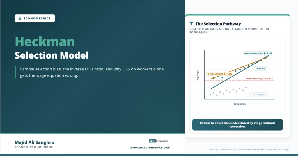
The two specifications agree on the qualitative pattern but diverge in magnitude on the variable that matters most. OLS on the workers gives an education return of 8.2 percent per year of schooling. The Heckman two-step gives 10.8 percent. The 2.6 percentage point gap is the selection correction: OLS was understating the return to education because the women who selected into the labor force at low education levels were a positively selected group, with unobserved characteristics that boosted their wages and partly compensated for their lower schooling. Once the Heckman model accounts for that selection, the structural return to education appears larger.

The inverse Mills ratio coefficient of 0.232 is statistically significant, confirming that selection is present. The positive sign indicates that unobserved factors raising the probability of working also raise observed wages. This is the typical finding in women’s labor supply studies of this kind, and it is the empirical pattern that motivated the Heckman framework in the first place.

The Logic Behind the Correction

The selection problem and its resolution can be visualized as a single picture. The latent wage offers in the population follow a distribution. So do the reservation wages, the threshold above which a woman chooses to work. A woman participates if her latent offer exceeds her reservation wage. The selection pattern is the relationship between these two distributions, and the Heckman correction is the formal procedure that recovers the unconditional offer distribution from the observed conditional one.

The figure makes the structural problem visible. The grey points are non-workers; their latent wage offers sit below the reservation wage threshold, and the data never observe these wages. The teal points are workers, and their wages enter the dataset. The teal regression line, fitted through the workers only, is flatter than the population regression line in teal, because the workers at low education levels are a positively selected group with above-average unobserved characteristics. The OLS estimate on workers therefore, understates the slope. The Heckman correction, by reconstructing the inverse Mills ratio for each observation, allows the wage equation to recover the steeper population slope.

Full-Information Maximum Likelihood

The two-step estimator is computationally simple and remains popular, but it is not the only way to estimate the Heckman model. The model can also be estimated by maximizing the joint likelihood of the participation indicator and the observed wage, treating both equations and the correlation parameter \(\rho\) as parameters to be estimated simultaneously. This is the full-information maximum likelihood (FIML) approach.

FIML is more efficient than the two-step estimator when the bivariate normality assumption holds, because it uses information from the joint density rather than estimating the two equations sequentially. The standard errors are also valid without the corrections that the two-step requires, since the two-step estimator inherits sampling variation from both stages and needs an asymptotic adjustment to produce correct standard errors. Modern software packages report FIML estimates as the default for the Heckman selection model, and the two-step estimator is increasingly reserved for cases where convergence problems with FIML force a more robust starting point. The general framework for likelihood-based estimation, including how the log-likelihood is constructed and maximized, is covered in the article on maximum likelihood estimation.

The trade-off between the two estimators is the standard one in econometrics. FIML wins on efficiency when the distributional assumption is correct. The two-step is more robust when normality is questionable, because the inverse Mills ratio enters the second-stage regression linearly and the wage equation coefficients are interpretable even if the joint normality assumption is approximate. In applied work that values transparency over efficiency, the two-step continues to dominate.

Limitations of the Heckman Model

The selection correction is sharp under its assumptions, and the assumptions are stronger than many users acknowledge. Three limitations deserve attention before the model is applied to a new dataset.

The first is the dependence on the bivariate normality assumption. The two-step estimator assumes the joint distribution of the participation and wage error terms is normal, and the inverse Mills ratio is derived from that distribution. When the true error distribution departs substantially from normality, the Mills ratio is misspecified and the second-stage coefficients are biased. Semi-parametric extensions of the Heckman model relax this assumption by estimating the selection correction term without a parametric distributional assumption, but they require larger samples and stronger exclusion restrictions to work well.

The second is the credibility of the exclusion restriction. The wage equation and the selection equation should differ in at least one variable, and that variable should plausibly affect participation without affecting wages directly. In the original women’s labor supply application, family structure variables provided that exclusion. In modern labor markets where employers offer parental benefits, where the presence of children may affect the kinds of jobs that women accept, and where the boundary between household production and market work is increasingly fluid, the exclusion restriction is harder to defend. A poorly justified exclusion restriction makes the Heckman estimates only nominally identified, and the wage coefficients can be highly sensitive to specification changes.

The third is the gap between selection correction and full causal identification. Correcting for selection bias makes the wage equation coefficients interpretable as the population return to characteristics among the observed group of workers. It does not address other sources of endogeneity in the wage equation, such as the possible correlation between education and unobserved ability. A Heckman correction combined with a careful identification strategy for the education coefficient, perhaps through an instrumental variable for schooling, is a stronger empirical design than either approach alone. The broader logic of identification, including how selection correction fits inside the modern causal inference toolkit, is the next layer of the discussion.

Applications Beyond Labor Economics

The Heckman model was developed for labor force participation, but its logical structure applies wherever the outcome of interest is observed only for a non-random subset of the population. Three application areas have absorbed the technique most thoroughly.

In development economics, household survey data on consumption or income are often observed only for households that respond to the survey, with non-response correlated with the very characteristics the researcher wants to study. Selection correction models adapted from Heckman’s framework address this problem in studies of poverty measurement and program evaluation.

In financial economics, returns are observed only for firms that survived the sample period, while delisted, bankrupt, or merged firms drop out of the data. Without correction, survivorship bias inflates the estimated return on equity strategies. The selection equation in this setting models the probability of survival, and the Mills ratio enters the return regression as a control. This logic generalizes to any setting where the analyst observes outcomes for surviving units only.

In education research, test scores are observed for students who completed the assessment, college outcomes are observed for students who enrolled, and earnings are observed for graduates who entered the labor market. Each of these conditional samples can be analyzed under a Heckman correction when an exclusion restriction is available, and the corrections often substantially change the estimated returns to educational interventions. Many of the same ideas inform modern work on gender gaps in labor force outcomes, where selection into work, into specific occupations, and into wage-bargaining settings remains central to interpreting the observed differences.

Explains

Conclusion

The Heckman selection model turned an intractable empirical problem into a tractable two-equation estimation procedure. By writing the outcome equation and the selection rule as a joint system with correlated error terms, Heckman showed that sample selection is a specific case of an omitted variable problem, and that the omitted variable can be reconstructed from a probit model of the selection decision. The inverse Mills ratio is the bridge between the two equations, and a significant coefficient on it in the second-stage regression is the empirical signature that selection bias is present.

The model’s continuing relevance rests on the credibility of its assumptions. The bivariate normality of the error terms and the existence of a defensible exclusion restriction are not formalities; they are the conditions under which the correction does the work it claims. When those conditions hold, the Heckman model recovers structural coefficients that are otherwise hidden behind the selection pattern of who enters the sample. When they fail, the correction can amplify the very biases it is intended to remove, and a carefully applied researcher will document the exclusion restriction, conduct sensitivity analysis on the distributional assumption, and report both the corrected and the uncorrected estimates.

The framework belongs alongside the wider toolkit of methods that handle non-random data in empirical econometrics, including instrumental variables for endogeneity, fixed effects for unobserved heterogeneity in panel data, and modern causal inference methods for treatment effects. Each of these techniques addresses a different way that observational data can mislead a researcher who runs OLS without thinking carefully about how the data were generated. The Heckman selection model addresses one specific way, and its 1979 formulation continues to shape how labor economists, development economists, and applied microeconometricians estimate wage equations, returns to schooling, and any outcome where who appears in the data is itself part of the economic story.

Frequently Asked Questions

Thanks for reading! If you found this helpful, share it with friends and spread the knowledge. Happy learning with MASEconomics