Hausman Test: Choosing Between Fixed and Random Effects

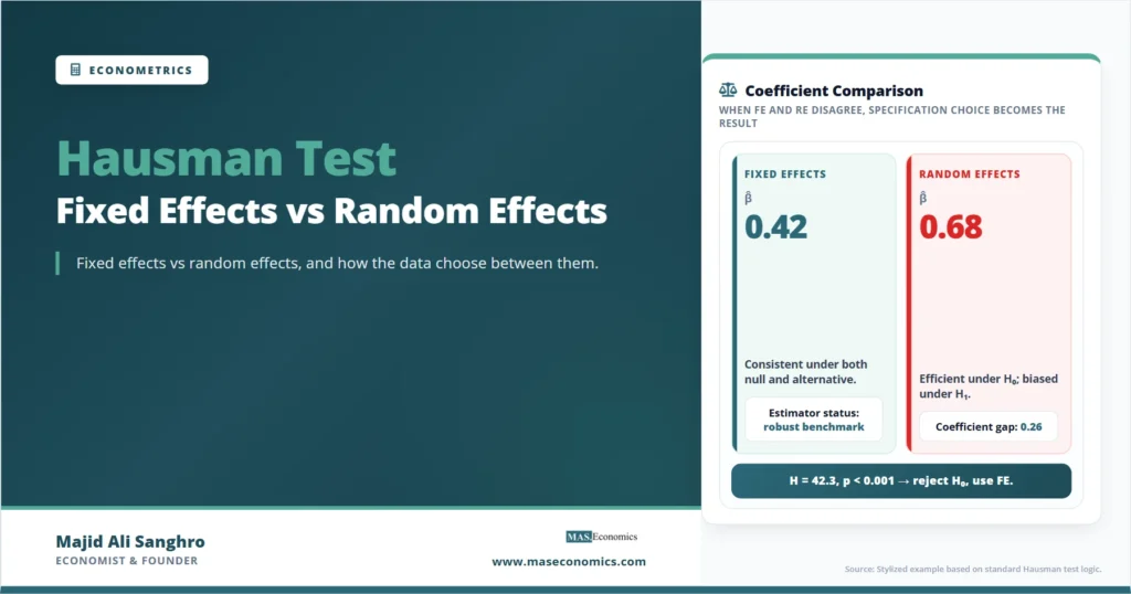
A labor economist analyzes twenty years of firm-level data on six thousand manufacturing companies. The central inquiry is whether a one percent rise in worker productivity translates into higher wages, and by how much. The data offer two estimators that look similar on the surface but rest on very different assumptions. A fixed effects estimator allows each firm to carry its own unobserved characteristics, such as a particular management style or capital vintage, and identifies the productivity-wage relationship from within-firm variation over time. A random effects estimator treats those firm-specific characteristics as random draws uncorrelated with productivity, and pools cross-sectional and time-series variation to produce a more efficient estimate. The two estimators give different coefficients. The Hausman test is the specification test that decides which set of assumptions the data support, and the choice has consequences for what the wage equation is allowed to claim.

Jerry Hausman’s 1978 paper in Econometrica formalized this kind of decision as a general comparison between two estimators: one that is consistent under both the null and alternative hypotheses, and one that is efficient under the null but inconsistent under the alternative. If the two estimators are statistically close, the efficient one wins. If they diverge by more than sampling error, the consistent one is the safer choice. The panel data version of this test, comparing fixed and random effects, is the most widely used application, and it sits at the center of how applied microeconometricians decide which model to report.

Panel Data Setup

Panel data follow the same units, such as firms, workers, households, or countries, over multiple time periods. The standard linear panel model can be written as:

Panel Regression

i indexes the unit (firm), t indexes the time period, u_i captures unobserved unit-specific heterogeneity, and ε_it is the idiosyncratic error.

The wage equation translates this notation into economics. Let \(y_{it}\) be log wages at firm i in year t, and let \(x_{it}\) be log productivity. The coefficient \(\beta\) is the productivity elasticity of wages. The term \(u_i\) represents everything about firm i that is constant over the sample, including management quality, location, capital vintage, union status, and industry niche. The term \(\varepsilon_{it}\) is the year-on-year shock that fluctuates around the firm’s average.

The challenge is that \(u_i\) is not observed. The econometrician has productivity, wages, and a firm identifier. What sits inside \(u_i\) is by definition not in the dataset. The Hausman test asks a precise question about that unobserved term: is it correlated with productivity, or is it not? The answer determines which estimator is consistent. The general structure of panel data, including the within and between variation that fixed and random effects exploit, is covered in the article on panel data econometrics.

Fixed Effects Estimation

The fixed effects estimator treats \(u_i\) as an unknown parameter for each unit and removes it through demeaning. For every firm, subtract the firm-specific time average from each observation:

Within Transformation

The unit-specific term u_i is constant over t, so it disappears when the firm mean is subtracted.

What survives is variation around each firm’s own average. The coefficient \(\hat{\beta}_{FE}\) is identified from how productivity and wages move together within firms over time, ignoring all between-firm differences. If Firm A has higher average productivity and higher average wages than Firm B, the fixed effects estimator does not use that comparison. It only uses the year-on-year movement of productivity and wages inside each firm.

The strength of this approach is that any time-invariant confounder, no matter how complex or unmeasured, is absorbed by the firm mean. Management quality could be heavily correlated with productivity, and the fixed effects coefficient on productivity is still consistent. The cost is efficiency. Throwing away between-firm variation means fewer degrees of freedom and noisier estimates, particularly when within-firm variation in productivity is small. The estimator also cannot identify the effect of any variable that does not change within firms over the sample, such as the firm’s founding industry or its country of incorporation.

Random Effects Estimation

The random effects estimator treats \(u_i\) as a random variable drawn from a population distribution, uncorrelated with the regressors. Under that assumption, the model becomes a generalized least squares problem with two error components, and the estimator combines within-firm and between-firm variation in a weighted average that minimizes variance.

Random Effects Composite Error

Identifying assumption: Cov(u_i, x_it) = 0 for all t. The unit effect is uncorrelated with the regressors.

If this assumption holds, the random effects estimator \(\hat{\beta}_{RE}\) is consistent and more efficient than fixed effects, because it uses the additional between-firm variation that fixed effects discards. It also estimates the coefficients on time-invariant variables, which fixed effects cannot.

The assumption is strong. In the wage equation, it requires that management quality, capital vintage, and every other unobserved firm characteristic be uncorrelated with productivity. That is rarely plausible. Firms with better management probably have higher productivity. Firms with newer capital vintages probably have higher productivity. If those characteristics also affect wages directly through bargaining, profit sharing, or selection of workers, the random effects estimator is biased. The bias does not shrink with sample size. It is a consistency problem, not a precision problem.

The Logic of the Hausman Comparison

The Hausman test exploits a structural feature of the two estimators. Under the null hypothesis that \(u_i\) is uncorrelated with the regressors, both estimators are consistent, but random effects is efficient and fixed effects is inefficient. Under the alternative hypothesis that \(u_i\) is correlated with the regressors, only fixed effects remain consistent, and random effects are biased.

Hausman’s insight was that under the null, the two estimators are estimating the same parameter, and their difference has a sampling distribution centered on zero. Under the alternative, the difference is centered on a non-zero quantity that reflects the bias in random effects. A statistical comparison of the two coefficient vectors therefore, identifies whether the null assumption is consistent with the data.

Hausman Statistic

Under H₀, H is asymptotically chi-squared distributed with k degrees of freedom, where k is the number of time-varying regressors compared.

The expression looks heavy, but the intuition is direct. The difference in coefficients is weighted by the inverse of the difference in variances. Under the null, both estimators converge to the same value, the variance of random effects is smaller than the variance of fixed effects, and the difference in variances is the correct scaling. The statistic asks: relative to the sampling noise we would expect under the null, is the gap between the two coefficient vectors larger than chance would explain?

A large H statistic means the two estimators disagree by more than sampling variation predicts. The null is rejected. The interpretation is that random effects is inconsistent because the unobserved heterogeneity is correlated with the regressors. Fixed effects is the safer choice. A small H statistic means the two estimators agree up to sampling noise. The null is not rejected, and random effects can be used because the efficiency gain comes without the cost of bias.

Wage-Productivity Example

Consider a stylized panel of 100 manufacturing firms observed annually for 15 years. The dependent variable is the log of average wages at the firm. The main regressor is the log of labor productivity. The question is what one decimal-point movement in log productivity does to log wages, and the two estimators give the following stylized output.

Table 1. Wage-Productivity Elasticity: Fixed Effects vs Random Effects

Specification	β̂ (productivity)	Std. error	Interpretation
Fixed effects (within)	0.42***	(0.05)	Within-firm pass-through
Random effects (GLS)	0.68***	(0.03)	Pooled within + between
Difference (FE – RE)	-0.26	(0.04)	Bias signal
Hausman statistic H	42.3	p < 0.001	Reject H₀
Source: Stylized example based on standard formulas. Significance: *** p < 0.01.

The two estimators give different answers. Random effects says a 1 percent rise in productivity is associated with a 0.68 percent rise in wages. Fixed effects says it is 0.42 percent. The gap of 0.26 percentage points is large in economic terms; it is the difference between a labor market with substantial productivity pass-through and one with moderate pass-through. The Hausman statistic of 42.3, evaluated against a chi-squared distribution with one degree of freedom, is far above any conventional critical value. The null of no correlation between firm-level heterogeneity and productivity is decisively rejected.

The economic interpretation is that something at the firm level, plausibly management quality, capital intensity, or worker selection, is driving both productivity and wages, and the random effects estimator was attributing this confounded variation to the productivity coefficient itself. The fixed effects coefficient of 0.42 reflects the genuine within-firm pass-through; the inflated random effects coefficient of 0.68 reflects bias. In an applied paper, the researcher reports the fixed effects estimate as the main result.

Hypotheses and Decision Rule

The Hausman test states a clean null and alternative, and the decision rule follows directly from the chi-squared critical value.

Hypotheses

Under H₀, both FE and RE are consistent; RE is efficient. Under H₁, only FE is consistent.

The test compares the H statistic to a chi-squared distribution with degrees of freedom equal to the number of time-varying regressors common to both specifications. If H exceeds the critical value at the chosen significance level, the null is rejected and fixed effects is selected. If H does not exceed the critical value, the null is not rejected and random effects can be used.

Table 2. Fixed Effects vs Random Effects: Decision Framework

Hausman result	Statistical reading	Estimator to report	Economic interpretation
H is small, p > 0.05	Cannot reject H₀	Random effects	Unit-specific heterogeneity is plausibly uncorrelated with regressors. RE is consistent and more efficient.
H is large, p < 0.05	Reject H₀	Fixed effects	Heterogeneity is correlated with regressors. RE is biased; FE is the consistent choice.
H is borderline	p between 0.05 and 0.10	Usually fixed effects	When in doubt, the consistent estimator is the safer report. Discuss both in robustness checks.
H is negative	Var(FE) < Var(RE) anomaly	Use robust variant	The asymptotic variance assumption has failed in finite samples. Use a robust or auxiliary regression version of the test.
Source: MASEconomics editorial synthesis based on Hausman (1978), Econometrica.

The decision framework is mechanical only when the assumptions of the standard Hausman test hold. The variance comparison in the denominator of H relies on the random effects estimator being efficient under the null, which requires homoscedastic and serially uncorrelated errors. When these assumptions fail, the standard statistic can be unreliable, and a robust variant is used instead. The same diagnostic logic that motivates the test for heteroscedasticity in the cross-sectional case applies here, and the standard treatment of heteroscedasticity in regression models carries over to the panel setting.

Connection to Endogeneity

The Hausman test belongs to a broader family of specification tests. The general principle is to compare two estimators where one is more efficient under the null and the other is more robust under the alternative, and to reject the null when the gap exceeds what sampling variation can explain. The same logic underlies the comparison between OLS and instrumental variables in the cross-sectional setting, where the question is whether an explanatory variable is correlated with the error term.

In the panel context, the unit effect \(u_i\) plays the role that the error term plays in cross-sectional endogeneity discussions. If \(u_i\) is correlated with the regressors, then conditioning on the random effects covariance structure does not eliminate the correlation, and the random effects estimator suffers from the same kind of inconsistency as OLS does in the presence of endogenous regressors. Fixed effects solves this by differencing out the source of correlation, just as instrumental variables address endogeneity in the cross-sectional case by isolating exogenous variation in the regressor.

The parallel is exact in structural terms. Random effects assume the unit effect is exogenous. Fixed effects do not require that assumption, at the cost of efficiency and the loss of any time-invariant coefficients. The Hausman test is the formal procedure that lets the data choose between these positions, and in most empirical labor and firm-level studies, the data choose fixed effects.

Variants and Robust Versions

The classical Hausman test described above assumes that the random effects estimator is efficient under the null. When errors are heteroscedastic or serially correlated, this assumption fails, and the variance difference in the denominator of H can become negative or unreliable. Several variants address this problem.

The most common modification is the auxiliary regression form. Construct the time-demeaned regressors and add both the demeaned variables and the original variables to a single regression. Under the null of random effects exogeneity, the coefficients on the demeaned variables should be statistically indistinguishable from zero. A Wald or F test on those auxiliary coefficients delivers the same inference as the classical Hausman statistic, and the test can be made robust to heteroscedasticity by using clustered or robust standard errors. This version is sometimes called the Mundlak or regression-based Hausman test, after Yair Mundlak’s 1978 article that proposed including unit means as additional regressors.

A second variant is the cluster-robust Hausman test, which replaces the variance matrices in the classical statistic with cluster-robust versions that allow for arbitrary correlation within firms. This is the form most commonly reported in modern applied work, especially with large panels where the homoscedasticity assumption is hard to defend.

A third variant is the bootstrap Hausman test, which constructs the sampling distribution of the H statistic by resampling firms with replacement and computing the test repeatedly. This approach is computationally heavier but avoids the asymptotic approximation altogether and gives reliable inference in smaller panels.

The choice among variants depends on the structure of the panel. For large panels with clear heteroscedasticity, the cluster-robust form is standard. For smaller or unbalanced panels, the bootstrap variant is more defensible. For pedagogical or quickly produced tests where the standard assumptions are roughly defensible, the classical form is the starting point. The principles behind these choices are also useful when working through econometric model selection more generally.

Limits of the Hausman Test

The Hausman test answers one question precisely: whether the data support the random effects assumption of orthogonality between the unit effect and the regressors. It does not decide several other things that applied researchers sometimes attribute to it.

It does not test whether unobserved heterogeneity exists at all. The presence of unit effects, fixed or random, is a separate question that is typically addressed with an F test on the unit dummies in the fixed effects specification or a Breusch-Pagan Lagrange multiplier test for random effects. The Hausman test takes for granted that some unit-level heterogeneity is present and only asks whether that heterogeneity is correlated with the regressors.

It does not test whether the linear panel model is correctly specified. If the true relationship is non-linear, if important interactions are omitted, or if the wrong variables are included, the Hausman test will still produce a statistic, but the statistic will not flag any of these problems. Functional-form misspecification is addressed by other diagnostics.

It does not test whether time effects belong in the model. The two-way model with both unit and time effects is a separate specification, and adding time effects can change the conclusion of the Hausman comparison. In modern applied work, the two-way fixed effects model is often the starting point, and the Hausman test is conducted within that framework rather than between it and a pooled model.

It does not establish causality. A rejection of the random effects assumption tells the researcher that fixed effects is the more consistent estimator, but the resulting fixed effects coefficient still requires that the regressor be uncorrelated with the time-varying idiosyncratic error \(\varepsilon_{it}\). If there is reverse causality between wages and productivity, or if a third time-varying factor drives both, the fixed effects estimate is still biased. The Hausman test selects the better estimator within the class of panel specifications; it does not settle identification.

Hausman Test in Modern Practice

In modern microeconometric practice, the Hausman test still appears in published work, but the decision it formalizes is often resolved on theoretical grounds before any test is conducted. The intuition is straightforward. In labor economics, firm-level studies, and most longitudinal household work, the unit-specific heterogeneity that random effects assumes away is almost always correlated with the regressors. Researchers therefore default to fixed effects, report a Hausman test for completeness, and interpret a non-rejection as a coincidence of small sample size rather than as evidence that random effects is appropriate.

This pattern reflects a deeper concern. The Hausman test has good power in large samples and against large violations, but it can fail to reject when the bias in random effects is moderate, and the sample is small. A non-rejection should therefore not be read as proof that random effects are safe. The economic logic of the application matters, and in most settings where firms or workers select into observed characteristics, the conservative choice is fixed effects regardless of what the test statistic says.

Where random effects continue to dominate is in cross-country panels with theoretical priors that the country effects are reasonably described as random draws, in studies where the time-invariant variables are themselves of central interest and fixed effects cannot identify them, and in longitudinal survey data where the random effects assumption is defensible as a starting approximation. In these settings, the Hausman test plays its original role as a discriminating tool. The companion estimation framework, including maximum likelihood estimation used to fit random effects under distributional assumptions, fits naturally into this decision.

Explains

Conclusion

The Hausman test formalizes the choice between fixed effects and random effects in panel data by comparing two estimators that rest on different assumptions about unobserved heterogeneity. Random effects is efficient when the unit-specific term is uncorrelated with the regressors, and biased otherwise. Fixed effects is consistent under both conditions but inefficient when the null holds. The test asks whether the gap between the two coefficient vectors exceeds what sampling variation predicts under the null, and a large statistic is read as evidence that the random effects assumption fails.

In applied work, the test sits inside a broader specification discipline that combines statistical diagnostics with economic reasoning. A rejection points to fixed effects as the consistent choice. A non-rejection does not automatically validate random effects, particularly in small panels or settings where firm or worker selection makes the orthogonality assumption hard to defend. The classical version of the test is now usually replaced by a robust variant that does not depend on the homoscedasticity assumption, and in many modern applications fixed effects is the default starting point with the Hausman test serving as confirmation rather than arbitration.

The test belongs to the larger family of specification comparisons in econometrics, alongside the OLS-versus-instrumental-variables comparison and the broader logic of econometric identification. Each of these procedures formalises the same underlying inquiry: when two estimators rest on different assumptions about the unobserved part of the model, the data can reveal which assumption is closer to the truth. The Hausman test gives that inquiry a precise answer in the panel setting, and the answer continues to shape how applied researchers report wage equations, firm performance regressions, and any model where the same units are followed over time.

Frequently Asked Questions

Thanks for reading! If you found this helpful, share it with friends and spread the knowledge. Happy learning with MASEconomics