Income Elasticity of Demand: Necessities, Luxuries, and Inferior Goods

Between 2010 and 2024, real disposable income in the United States rose by roughly 25 percent. Over the same period, household spending on restaurant meals rose by 60 percent. Spending on canned soup, by contrast, fell. Both numbers come from the same households facing the same prices, and the only thing that changed was how much money they had to spend. The economic concept that explains why one category soared while another shrank is the income elasticity of demand, the single measure that classifies goods as necessities, luxuries, or inferior, and that drives nearly every empirical model of household consumption.

The idea traces back to Ernst Engel’s 1857 study of Belgian working-class budgets, where he documented that the share of income spent on food declines as households grow richer. That regularity, now called Engel’s Law, became the foundation for one of the most-used parameters in applied economics. Where price elasticity asks how consumers respond to a change in what something costs, income elasticity asks how they respond to a change in what they can afford. The two questions are different. The answers often point in different directions, and the policy implications diverge accordingly.

What Income Elasticity of Demand Measures

Income elasticity of demand (YED) is the percentage change in quantity demanded of a good divided by the percentage change in consumer income:

INCOME ELASTICITY OF DEMAND

The sign and magnitude of YED classify a good as normal (positive YED), inferior (negative YED), a necessity (0 < YED < 1), or a luxury (YED > 1).

The interpretation hinges on the sign. A positive YED means demand grows with income, which describes most goods in most economies. A negative YED means demand shrinks as income rises, which describes a smaller category of goods that households replace with higher-quality alternatives once they can afford to. Magnitude then refines the picture: among normal goods, some are necessities that households buy slightly more of when richer (food, basic clothing), while others are luxuries that households buy much more of (international travel, fine dining, second homes).

The formula is structurally identical to the price elasticity of demand and supply, but the comparison is between quantity and income rather than quantity and price. Both elasticities are unit-free percentage ratios, which is what makes them comparable across goods, countries, and time periods.

A Worked Example

The cleanest way to anchor the formula is with a concrete calculation. Suppose average household income in a city rises by 10 percent over the year. A luxury car dealership records annual sales rising from 500 units to 600 units, a 20 percent increase. The YED for these vehicles is:

A YED of 2.0 indicates a luxury normal good. As households grow richer, their purchases of luxury cars grow at twice the rate of their income. The interpretation matters for the dealership’s business model. In an expanding economy, their volume grows faster than the underlying customer base. In a contracting one, it shrinks faster. The same YED that makes luxury cars a great business in good times makes them a fragile business in bad ones.

Now consider the opposite case. Suppose the same 10 percent income increase coincides with a 5 percent drop in sales of instant ramen noodles. The YED is:

A negative YED of −0.5 indicates an inferior good. As households grow richer, they buy less ramen and substitute toward higher-quality meals. The good itself is not defective. It is simply lower on a quality ladder that consumers climb when their income permits. Public transportation, generic store-brand groceries, and used clothing typically show similar patterns in cross-sectional data.

The Four Categories of Goods

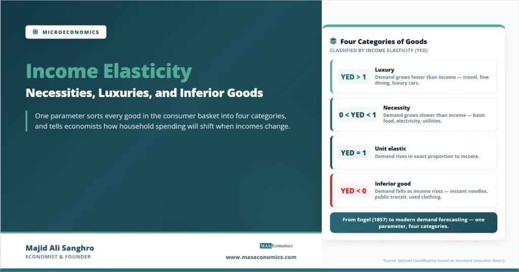
The YED value sorts every good in the consumption basket into one of four classes. Each carries different implications for pricing strategy, government policy, and economic forecasting.

Table 1. Classification of Goods by Income Elasticity

YED value	Classification	Income response	Typical examples
YED < 0	Inferior good	Demand falls as income rises	Instant noodles, public transit, second-hand clothing, generic-brand staples
0 < YED < 1	Necessity (normal good, income-inelastic)	Demand rises with income, but less than proportionally	Basic food, electricity, utilities, primary healthcare
YED = 1	Unit elastic normal good	Demand rises in exact proportion to income	Mid-tier discretionary spending in some empirical studies
YED > 1	Luxury (normal good, income-elastic)	Demand rises faster than income	International travel, fine dining, luxury vehicles, premium electronics
Source: MASEconomics editorial synthesis based on standard consumer theory and applied econometric estimates.

The boundary at YED equal to one separates necessities from luxuries within the normal-goods category, and the boundary at zero separates normal goods from inferior goods. These two thresholds carry most of the analytical weight. A YED that crosses zero indicates that consumer preferences have shifted enough to make the good less desirable as income rises. A YED that crosses one indicates that the good has moved from the necessity tier into the luxury tier, or vice versa, which often happens as economies develop and once-aspirational items become standard household possessions.

Engel’s Law and the Original Empirical Anchor

The strongest empirical regularity in income elasticity is also the oldest. In 1857, the German statistician Ernst Engel analyzed budget data from working-class families in Belgium and observed that the share of household spending devoted to food falls as household income rises. Richer families spend more on food in absolute terms, but food consumes a smaller fraction of their total budget. The implied income elasticity for food is positive but less than one, placing it firmly in the necessity category.

Engel’s Law has been replicated in nearly every country and every decade since, with remarkable consistency. The US Bureau of Labor Statistics Consumer Expenditure Survey shows the bottom income quintile spends around 33 percent of its income on food, while the top quintile spends around 8 percent. The income elasticity for food in modern US data runs between 0.3 and 0.5, depending on the food category and the time period.

The same logic extends beyond food. As economies develop, the income share spent on housing, clothing, and basic services tends to decline while the share spent on entertainment, travel, education, and discretionary services rises. This pattern is so reliable that the long-run shift in household consumption composition is sometimes called the Engelian transition, and it underlies forecasts of how emerging-market consumer demand will reshape global trade flows over the coming decades.

Why the Same Good Can Have Different Income Elasticities

One of the most useful insights from applied work is that YED is not a fixed property of a good. The same product carries different income elasticities depending on context. Three factors do most of the work.

The income level of the consumer. A car may be a luxury for a household in a developing economy and a necessity for a household in a high-income one. At low income levels, owning a vehicle is aspirational and YED is high. At high income levels, vehicle ownership is near-universal and additional income buys a better vehicle rather than another one, lowering YED. This is why YED estimates from developing-country data and developed-country data often differ for the same nominal category.

The point on the consumer’s quality ladder. Many goods exist on a quality continuum. As income rises, households trade up to higher-quality versions of the same broad category. Ground beef has positive YED at low income levels, then becomes inferior as households shift to steak. Public transit has positive YED in early development, then becomes inferior as private cars become affordable. The transition point depends on relative prices, cultural preferences, and infrastructure.

The time horizon. Short-run YED estimates are typically smaller than long-run ones because consumption habits adjust slowly. A household that receives a permanent income increase may maintain its previous consumption pattern for months or years before fully adjusting. Long-run YED captures the steady-state response after habits, durables, and housing decisions have re-optimized to the new income level.

Estimating YED from Real Data

The empirical estimation of income elasticity is more complicated than the formula suggests. Three difficulties recur across applied studies.

The first is that income and prices often move together. A household whose income rises may also face different prices because they shop at different stores, buy in different quantities, or face different regional price levels. Separating the pure income effect from confounding price effects requires careful identification, usually through panel data or instrumental variables.

The second is the choice of income measure. Current income, permanent income, and household wealth all carry different implications for consumption decisions. Milton Friedman’s permanent income hypothesis argued that households smooth consumption against expected lifetime income rather than reacting to short-run income shocks, which means YED estimated against current income may understate the structural response. Long-run YED estimates that use multi-year income averages are typically larger than year-on-year estimates.

The third is heterogeneity. YED differs across age groups, household compositions, education levels, and regions. Pooled estimates conflate these subgroups, sometimes producing misleading aggregate values. Modern studies use household-level microdata from consumer expenditure surveys to estimate YED separately for population segments. The Consumer Expenditure Survey in the United States, the Living Costs and Food Survey in the United Kingdom, and similar instruments elsewhere are the standard data sources.

Why YED Matters for Business and Policy

Income elasticity is one of the most consequential parameters in applied economics because it determines how household consumption shifts over the business cycle and across long-run development paths.

Business cycle forecasting. When a recession reduces household income by five percent, demand for goods with high YED falls disproportionately. The 2008 to 2009 financial crisis cut US household income by roughly four percent in real terms and produced a 20 percent drop in luxury goods spending, a 12 percent drop in restaurant meals, and a four percent drop in groceries. The differential response is exactly what YED predicts. Firms in high-YED categories face amplified cyclicality, while firms in low-YED categories see steadier demand through downturns.

Tax policy and incidence. Governments designing progressive taxation often use YED estimates to predict how tax changes affect consumption patterns. A luxury tax on high-YED goods raises revenue mostly from higher-income households, since they consume those goods disproportionately. A subsidy on low-YED necessities reaches lower-income households more efficiently, since those goods make up a larger share of their budgets. Misjudging YED produces taxes that fail to hit their intended target.

Long-run development planning. As emerging economies grow, the composition of consumer demand shifts predictably along the lines Engel identified. Demand for basic foods grows slowly, demand for processed foods and dining out grows faster, and demand for travel, healthcare, education, and entertainment grows fastest. Firms expanding into developing markets and governments planning infrastructure investment both rely on YED estimates to anticipate which sectors will grow as incomes rise.

Trade and global demand patterns. Goods with high YED account for a disproportionate share of growth in global trade as middle-class populations expand. The rise of consumer-class spending in China and India over the past two decades has driven outsized growth in international tourism, luxury goods, premium electronics, and high-protein food categories, all consistent with the YED predictions made decades earlier.

Common Mistakes to Avoid

Three mistakes recur often enough to flag explicitly.

The first is confusing income elasticity with price elasticity. The two are different parameters that answer different questions. A good can be price-inelastic (consumers buy nearly the same quantity when price changes) while being income-elastic (consumers buy much more when income changes). Healthcare is one example: largely insensitive to price at the point of consumption due to insurance coverage, but highly responsive to long-run income trends. Quoting one elasticity when the other is the relevant parameter is a frequent source of analytical error.

The second is treating the inferior-good label as a quality judgment. An inferior good is not a low-quality good. It is a good whose consumption falls as income rises. Public transit in a wealthy city may be high quality and still show negative YED, simply because higher-income residents prefer driving. The economic classification reflects the consumption-income relationship, not the intrinsic merits of the product.

The third is assuming YED is stable over time. Goods migrate across categories as economies develop, technologies change, and preferences shift. Air travel was a luxury with YED above two in the 1970s. It has become a necessity in many high-income countries for business and family travel, with YED closer to 0.5 in current data. Long-range forecasts that hold YED constant typically overstate growth in goods that have already saturated and understate growth in goods entering the discretionary tier for the first time.

Explains

Conclusion

The income elasticity of demand sorts every good in the consumer basket into one of four categories and tells economists how household consumption patterns will shift when incomes change. The mathematical machinery is simple, a percentage change ratio, but the empirical insight is rich. Necessities grow slowly with income. Luxuries grow faster. Inferior goods shrink. These three regularities, anchored by Engel’s 1857 observation about food spending, organize a remarkable amount of consumer behavior across countries and decades.

The number is useful most of all because it disciplines forecasting. Business cycle predictions, tax incidence analysis, long-run development planning, and global demand modeling all rely on YED estimates to anticipate how household choices will respond to income changes. The estimates themselves vary across contexts, time horizons, and subgroups, which means careful empirical work is required to apply them well. What does not vary is the underlying logic. Households climb a quality ladder as they grow richer, shedding some goods, adopting others, and reshaping the composition of demand in the process. Engel was the first to document this rigorously. Modern applied economics still rests on the parameter he identified.

Frequently Asked Questions

Thanks for reading! If you found this helpful, share it with friends and spread the knowledge. Happy learning with MASEconomics