Households do not spend based solely on their current paycheque. A worker earning a high salary in their fifties does not consume proportionally more than a young adult borrowing to fund education, nor an octogenarian drawing down retirement savings. In 1954, Franco Modigliani and Richard Brumberg proposed a framework that transformed how economists understand consumption and saving. The life-cycle hypothesis posits that individuals plan their consumption and saving behaviour over their entire lifespan, smoothing their standard of living rather than matching spending to period-by-period income. This insight resolved inconsistencies in the simple Keynesian consumption function, which posited that current consumption depends only on current income, and it provided a microeconomic foundation for understanding national saving rates, capital accumulation, and the macroeconomic effects of fiscal policy.
Before Modigliani and Brumberg, the dominant view was that households consumed a fixed proportion of their current disposable income. This assumption created empirical problems, particularly the failure of aggregate consumption to fall as much as predicted during temporary income shocks like the Great Depression. The consumption function needed a forward-looking dimension. The life-cycle hypothesis supplied it by placing the lifetime budget constraint at the centre of the analysis. Households are not passive responders to current income; they are intertemporal optimisers, borrowing against future earnings when young, accumulating wealth during peak earning years, and decumulating that wealth in retirement. This lifecycle pattern has profound implications for how economies respond to tax cuts, pension reforms, and demographic shifts.
The Logic of Life‑Cycle Saving
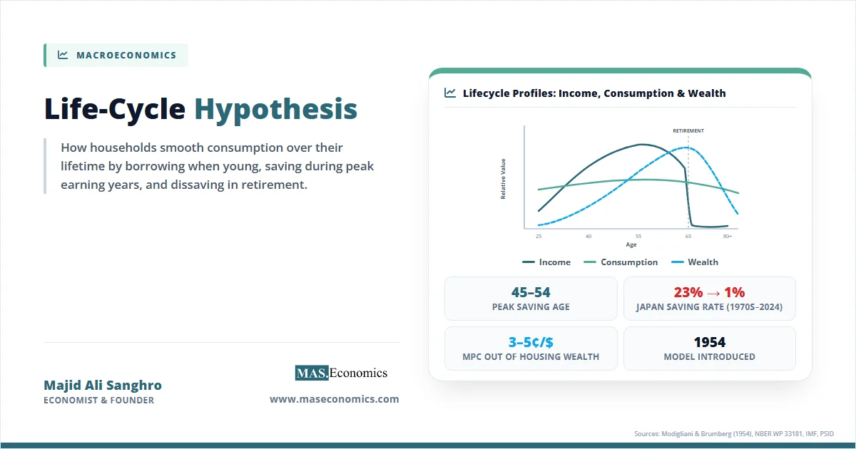
The central premise of the life-cycle hypothesis is consumption smoothing. Individuals derive utility from consumption, and because the marginal utility of consumption diminishes, a stable consumption path yields higher lifetime utility than a volatile one that tracks the natural hump shape of income over a lifetime. A typical worker experiences low income in early adulthood, rising income through middle age, and a sharp decline in income at retirement. If consumption tracked income exactly, the individual would consume very little when young and old, and a great deal in middle age. Instead, households use financial markets to reallocate resources across time.
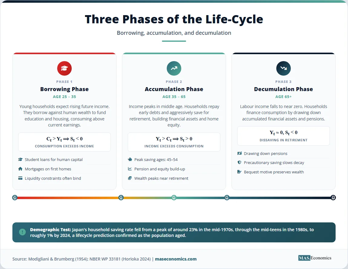
The lifecycle can be divided into three distinct phases. In the first phase, early adulthood, individuals expect their future income to rise. To smooth consumption, they borrow or dissave, spending more than they earn. This behaviour explains why young households take on student loans, mortgages, and credit card debt. In the second phase, middle age, income peaks. Households repay their early debts and save for retirement, accumulating financial assets. This saving takes the form of pension contributions, home equity, and investment portfolios. In the third phase, retirement, labour income falls to zero or near zero. Households finance their consumption by drawing down the wealth accumulated during the second phase, a process called dissaving. At the end of life, the model assumes wealth is exhausted, a condition known as the zero-bequest assumption.
This framework generates clear, testable predictions about the relationship between age, income, and wealth. Wealth should follow an inverted U-shape over the lifetime, peaking at the age of retirement and declining thereafter. Saving rates should be negative for the young and the old, and positive for the middle-aged. Aggregate saving rates in a country should depend on the age structure of the population: economies with a large working-age population should save more than economies with a high proportion of elderly citizens. These predictions shifted the analysis of saving from a purely static exercise to a dynamic, demographic one.
The life-cycle hypothesis also provides a distinct theory of the wealth-consumption relationship. Because consumption depends on lifetime resources, which include both current income and accumulated wealth, an increase in asset values, such as a rise in stock prices or housing values, should increase consumption even if current income remains unchanged. This wealth effect became a central mechanism in modern macroeconomic models, particularly in explaining the consumption booms of the 1990s and 2000s, when rising asset prices fuelled spending without corresponding income growth. The macroeconomic models that central banks use today incorporate this wealth effect directly.
The Life‑Cycle Hypothesis in Equations
The formalisation of the life-cycle hypothesis begins with an individual who lives for \( T \) periods and maximises lifetime utility, subject to an intertemporal budget constraint. The objective function is the discounted sum of period-by-period utility from consumption \( C_t \):
where \( u(\cdot) \) is a strictly increasing, strictly concave period utility function, and \( \beta = \frac{1}{1+\rho} \) is the discount factor, with \( \rho \) being the subjective rate of time preference. A higher \( \rho \) implies that the individual is less patient, weighting present consumption more heavily relative to future consumption.
The individual faces an intertemporal budget constraint that equates the present discounted value of lifetime consumption to the present discounted value of lifetime resources, which consist of initial wealth \( A_0 \) and labour income \( Y_t \) earned over \( R \) working years. Assuming a constant real interest rate \( r \), the constraint is:
Under the assumption that the interest rate equals the rate of time preference (\( r = \rho \)), the individual chooses to consume an equal amount in every period. This is the complete consumption smoothing result. Let \( W \) denote total lifetime resources, defined as the sum of initial wealth and the present value of future labour income, often called human wealth. The optimal consumption path is:
More explicitly, the consumption function can be expressed as a linear function of wealth and current income. In a simplified version of the model, the aggregate consumption function takes the form:
where \( A_t \) is non-human wealth (financial assets and housing), \( Y_t \) is current labour income, and \( Y_t^e \) is expected future labour income. The parameters \( \alpha \), \( \beta \), and \( \gamma \) depend on the interest rate, the time horizon, and the specific utility function. The key insight is that the marginal propensity to consume out of current income \( \beta \) is not unity, as the simple Keynesian model would suggest. Instead, \( \beta \) is small, because current income is only one component of total lifetime resources. A temporary change in income, such as a one-time tax rebate, is spread over the entire remaining lifetime, so its impact on current consumption is negligible. This prediction distinguishes the life-cycle hypothesis sharply from models where consumption tracks current income.
The evolution of wealth is determined by the saving decision. Saving \( S_t \) is defined as the difference between income and consumption. For a working individual:
During the working years, \( Y_t > C_t \), so \( S_t > 0 \) and wealth accumulates. During retirement, \( Y_t = 0 \), so \( S_t = -C_t \) and wealth decumulates. The path of wealth over the lifetime is:
with the terminal condition \( A_T = 0 \), ensuring that the individual dies with no unused resources. The table below summarises the key variables and their roles in the mathematical formulation.
| Variable | Definition | Role in the Model |
|---|---|---|
| \( T \) | Lifespan (number of periods) | Defines the planning horizon over which the individual optimises |
| \( C_t \) | Consumption in period t | The choice variable that the individual maximises utility over |
| \( Y_t \) | Labour income in period t | Zero after retirement; core component of lifetime resources |
| \( A_t \) | Non-human wealth in period t | Accumulates during working years, decumulates in retirement |
| \( \beta \) | Subjective discount factor | Determines the relative weight of present vs. future consumption |
| \( r \) | Real interest rate | Return on saved wealth; affects the intertemporal price of consumption |
| \( W \) | Total lifetime resources | Sum of initial wealth and the present value of future labour income |
 | ||
Key variables in the mathematical formulation of the life-cycle hypothesis. The model predicts that consumption depends on total lifetime resources \( W \), not solely on current income \( Y_t \).
Key Assumptions and Limitations of the Model
The life-cycle hypothesis relies on several strong assumptions that limit its empirical accuracy and theoretical completeness. Understanding these boundaries is necessary for evaluating the model’s predictions and the validity of its policy implications.
The first key assumption is the existence of perfect capital markets. The model assumes individuals can borrow freely against their future labour income at the prevailing interest rate. In reality, borrowing constraints are pervasive, especially for young households. A recent graduate with high expected future earnings cannot necessarily borrow to smooth consumption today because lenders cannot perfectly enforce repayment, and human capital cannot be seized as collateral. These liquidity constraints force young individuals to consume less than the model predicts, violating the consumption smoothing result. Empirical work by Zeldes (1989) and others has shown that liquidity-constrained households exhibit a much higher marginal propensity to consume out of current income than unconstrained households, a finding consistent with rule-of-thumb consumers who simply spend their current income.
The second major assumption is the absence of uncertainty. The basic formulation assumes individuals know their lifespan, their future income trajectory, and the rate of return on their assets with certainty. In the real world, all three are uncertain. People face longevity risk, the possibility of outliving their savings; income risk from unemployment, illness, or sectoral shifts; and return risk on their investment portfolios. The introduction of uncertainty, particularly uninsurable income shocks, fundamentally alters the saving decision. Households save not only to smooth consumption over the expected lifecycle, but also as a precaution against adverse shocks. This precautionary saving motive explains why the elderly often do not accumulate their wealth as rapidly as the deterministic model predicts. They hold onto assets as a buffer against the risk of high medical expenses or the possibility of living longer than expected. The precautionary saving channel, formalised by Caballero (1990), adds a substantial wealth accumulation component that the basic model misses.
Third, the model assumes a zero-bequest motive. Individuals are assumed to derive utility only from their own consumption and to die with exactly zero wealth. While analytically convenient, this assumption is strongly contradicted by data. A significant fraction of aggregate wealth is held by elderly households that do not spend it down, and a substantial portion of this wealth is ultimately bequeathed to heirs. If individuals value the welfare of their descendants, or if they derive utility directly from leaving a legacy, their optimal consumption path will be lower at every age, and they will not fully decumulate their wealth in retirement. The bequest motive changes the relationship between age and wealth, flattening the dissaving phase. It also alters the fiscal implications of the model, because tax policy that affects the after-tax return on capital must account for the desire to transfer wealth intergenerationally.
Fourth, the model abstracts from behavioural biases and bounded rationality. Solving the intertemporal optimisation problem requires significant cognitive effort and self-control. Households must estimate their lifespan, project their income decades into the future, and calculate the appropriate saving rate. Behavioural economists have documented widespread present bias, where individuals systematically overvalue immediate consumption relative to future consumption, leading to undersaving. This myopia implies that many households arrive at retirement with insufficient wealth, relying heavily on government pensions and transfers rather than their own accumulated assets. The gap between the rational optimiser of the life-cycle model and actual human behaviour has driven the rise of behavioural economics explanations of saving, including automatic enrolment in pension plans and default contribution rates.
Finally, the aggregation from individual to macroeconomic saving rates presents difficulties. The model predicts that aggregate saving depends on the age structure of the population. However, the empirical link between demographics and saving rates is complicated by economic growth. If the economy is growing, younger generations are richer than older generations, and the aggregate dissaving of the elderly is offset by the higher savings of the young. Modigliani himself noted that aggregate saving rates depend on the growth rate of the economy, not just the demographic composition. In a stationary economy, the saving of the working population exactly offsets the dissaving of the retired, resulting in a net aggregate saving rate of zero. It is economic growth that generates positive aggregate saving, because the young, who are richer in lifetime terms, save more than the old, who dissave.
Empirical Evidence for Life‑Cycle Saving
Testing the life-cycle hypothesis requires data on consumption, income, and wealth across different age cohorts. The broad patterns in the data support the model’s qualitative predictions, but the quantitative deviations are significant. Income does follow a hump shape over the lifetime, peaking in the fifties and declining sharply at retirement. Consumption also follows a hump, but it is notably flatter than the income profile, consistent with the consumption smoothing hypothesis. Households do save during their working years and do draw down assets in retirement. However, the extent of dissaving among the elderly is less than the basic model predicts, a phenomenon known as the retirement saving puzzle.
The chart below illustrates the stylised lifecycle profiles for income, consumption, and wealth. The income profile rises through early and middle adulthood before falling at retirement. The consumption profile is smoother, supported by borrowing in early adulthood and dissaving in retirement. The wealth profile shows accumulation during working years, peaking near retirement age, followed by a gradual decline.
Stylised lifecycle profiles of income, consumption, and wealth relative to their peak values. Income (primary teal) shows a steep hump, while consumption (secondary mint) is smoothed across the lifetime. Wealth (blue) peaks near retirement and declines gradually, reflecting the life-cycle hypothesis.
Empirical studies using household survey data, such as the Panel Study of Income Dynamics in the United States and the English Longitudinal Study of Ageing, confirm these broad patterns but reveal important nuances. A key finding is that the wealth profile does not decline as steeply after retirement as the pure model predicts. Hurd (1987) showed that while single retirees do dissave, the rate of decumulation is slow, and couples often maintain or increase their wealth well into their seventies. This anomaly is partly explained by the bequest motive, partly by precautionary saving against medical expenditure shocks, and partly by the desire to remain in the family home, an illiquid asset that is costly to convert into consumption.
The model’s prediction regarding the aggregate saving rate has also been tested across countries. According to the hypothesis, countries with rapidly growing populations should have higher saving rates, because a larger proportion of the population is in the high-saving, middle-aged cohort. Conversely, countries with aging populations should experience declining saving rates. International Monetary Fund research has found a robust negative correlation between the old-age dependency ratio and the national saving rate, consistent with the life-cycle prediction. Japan, one of the most rapidly aging societies, has seen its household saving rate fall from a peak of roughly 23% in the mid-1970s, through the mid-teens in the 1980s, to about 1% by 2024 (Horioka 2024). The demographic transition currently underway across the developed world provides a large-scale, ongoing test of the model’s macroeconomic implications.
Cross-sectional tests offer further support. The marginal propensity to consume out of a temporary income shock should be small, close to the annuity value of the shock. Studies of the 2008 and 2020 fiscal stimulus payments in the United States found that households spent between one-third and one-half of the rebates within the first few months, a figure higher than the pure model predicts but lower than a simple Keynesian consumption function would suggest. This pattern points to the presence of both life-cycle planners and liquidity-constrained rule-of-thumb consumers in the population. The permanent income hypothesis, a close cousin of the life-cycle model, provides the theoretical benchmark for interpreting these estimates.
The table below contrasts the life-cycle hypothesis with the alternative major theories of consumption, highlighting how each framework treats the relationship between income and consumption.
| Feature | Keynesian Absolute Income | Life-Cycle Hypothesis | Permanent Income Hypothesis |
|---|---|---|---|
| Primary determinant of consumption | Current disposable income | Lifetime resources (wealth + current + future income) | Permanent income |
| Marginal propensity to consume (temporary income shock) | High (near 1) | Low (spread over lifetime) | Low (spread over lifetime) |
| Wealth profile over lifetime | Not modelled | Hump-shaped, peaks at retirement | Depends on permanent income shocks |
| Key demographic implication | None | Saving rate depends on age structure | Saving rate depends on income growth |
| Role of borrowing constraints | Not modelled | Violates smoothing for the young | Creates rule-of-thumb consumers |
| |||
Comparison of major consumption theories. The life-cycle hypothesis and permanent income hypothesis share a forward-looking orientation but differ in their emphasis on age-specific wealth accumulation versus permanent income estimation.
How the Life‑Cycle Hypothesis Shapes Policy
The life-cycle hypothesis is not merely a theoretical description of individual behaviour; it is a workhorse model for macroeconomic policy, fiscal analysis, and financial planning. Its implications affect how governments design tax systems, how central banks evaluate the transmission of monetary policy, and how societies prepare for the fiscal consequences of demographic change. The model’s central insight, that consumption depends on lifetime resources rather than current income, reshapes the analysis of almost every major macroeconomic policy question.
Consider the design and evaluation of fiscal stimulus. During a recession, governments often cut taxes or issue rebate cheques to boost household spending. The effectiveness of these measures depends critically on the marginal propensity to consume out of the transfer. If households behave according to the simple Keynesian consumption function, a one-dollar tax cut generates nearly one dollar of immediate spending. If households behave according to the life-cycle model, a temporary tax cut is perceived as a small addition to lifetime resources, and the marginal propensity to consume is close to the annuity value of that addition. For a working-age household with a long remaining horizon, a $1,000 rebate might increase current consumption by only $30 to $50. The rest is saved. This prediction explains why temporary tax rebates, such as those implemented in the United States in 2001, 2008, and 2020, typically produce a modest and short-lived boost to aggregate demand. A permanent tax cut, by contrast, has a much larger effect on perceived lifetime resources and thus on consumption. The fiscal policy implications are clear: the timing and duration of tax changes matter enormously, and one-off transfers are an inefficient way to stimulate spending among unconstrained households.
The hypothesis also provides the intellectual foundation for understanding wealth effects and the monetary policy transmission mechanism. When central banks lower interest rates, asset prices typically rise. Higher equity and housing values increase household wealth, which, according to the life-cycle consumption function, should boost spending even if current income is unchanged. The marginal propensity to consume out of wealth is estimated to be between 3 and 5 cents per dollar for housing wealth, and 2 to 3 cents per dollar for financial wealth. While these coefficients are small, the sheer size of aggregate housing and stock market wealth means that wealth effects can have a significant macroeconomic impact. During the housing boom of the early 2000s, rising home equity supported robust consumption growth. When the bubble burst, the destruction of household wealth contributed to the sharp contraction in spending during the Great Recession. Central banks monitor these wealth channels closely, and the life-cycle model provides the theoretical framework for interpreting the data. The fiscal multiplier is substantially larger in economies where wealth effects are weak and liquidity constraints are prevalent because a higher fraction of households live hand-to-mouth.
Demographic change is perhaps the most important domain where the life-cycle hypothesis informs current policy debates. Populations in Japan, Europe, and increasingly China are aging rapidly. The old-age dependency ratio, the number of people over 65 relative to those of working age, is rising sharply. According to the model, this demographic shift should reduce aggregate saving rates, because a larger fraction of the population is in the dissaving phase of life. Lower national savings means less domestic capital available for investment, putting upward pressure on real interest rates, all else equal. It also means a smaller tax base to fund the pensions and healthcare costs of the elderly. The interaction between demographics and inflation is an active area of research, with some economists arguing that aging populations are inherently disinflationary because they consume less and demand fewer goods, while others point to the rising cost of services like healthcare. The life-cycle framework provides the structural link between population aging, national saving, and capital flows. Countries with young populations, such as India, should be net savers and capital exporters, while aging countries, such as Japan, should be capital importers. The global pattern of imbalances partly reflects these lifecycle differences across nations.
Pension system design is another area where the model is indispensable. The shift from defined benefit pensions, which guarantee a fixed income in retirement, to defined contribution plans, which place the investment and longevity risk on the individual, has made lifecycle saving behaviour more important than ever. In a defined contribution system, individuals must decide how much to save during their working years and how quickly to draw down their assets in retirement. The life-cycle model prescribes an optimal path, but behavioural evidence shows that many individuals fail to save enough, suffer from inertia, and make poor investment choices. This gap between the theoretical optimum and actual behaviour has driven regulatory interventions, such as automatic enrolment in employer-sponsored plans and required minimum distributions from retirement accounts after age 72. These policies are designed to nudge behaviour closer to the lifecycle optimum.
The model’s implications extend to the analysis of income inequality and redistribution. Because consumption smoothing implies that households spread their lifetime resources evenly, annual income is a poor measure of welfare. A medical student with low current income but high expected future earnings is not poor in the lifecycle sense. Conversely, a retiree with high wealth but low current income is not poor either. The life-cycle perspective suggests that policies aimed at redistribution should account for lifetime income, not just point-in-time income. A tax system that penalises high earners during their peak earning years but ignores the decades of low income they experienced earlier may be more distortionary than a system based on lifetime earnings. Several European countries have explored lifetime income averaging for tax purposes, an idea directly rooted in the life-cycle framework.
Furthermore, the hypothesis informs the analysis of government debt and intergenerational accounting. Government debt represents a claim on future taxpayers. The life-cycle model shows that the burden of debt depends on how it affects the lifetime budget constraints of different generations. If the government borrows today and raises taxes tomorrow, it shifts resources from younger, future taxpayers to older, current bondholders. This intergenerational transfer can reduce national savings if the elderly have a higher marginal propensity to consume out of government transfers than the young have to reduce their consumption in anticipation of future taxes. The framework provides the analytical tools to evaluate the long-run fiscal sustainability of sovereign debt and entitlement programmes.
MASEconomics Explains
Four economic concepts behind the life-cycle hypothesis
Conclusion
The life-cycle hypothesis remains the foundational framework for understanding how households allocate consumption and saving across their lifetimes. By placing the intertemporal budget constraint at the centre of the analysis, Modigliani and Brumberg showed that current income is only one component of the spending decision, and that forward-looking households smooth their consumption by borrowing when young, saving during peak earning years, and dissaving in retirement. While the basic model abstracts from uncertainty, liquidity constraints, and bequest motives, its core logic drives modern macroeconomic policy, from the design of fiscal stimulus and pension systems to the analysis of demographic change and wealth effects. Empirical evidence supports the broad predictions of consumption smoothing and age-dependent wealth accumulation, even as it reveals important deviations that have enriched the theory. As populations age and the responsibility for retirement saving shifts to individuals, the insights of the life-cycle hypothesis are more relevant than ever.
Did you find this article helpful? Share it with someone who loves economics. And remember, at MASEconomics, we make complex ideas simple.