Ask people how many years of schooling they completed and about one answer in ten is wrong, sometimes by a year, sometimes by more. Regress wages on those answers and the estimated return to a year of schooling comes out too small, by roughly the share of the answers that were noise. That is attenuation bias, the oldest and most reliable failure in applied econometrics: a regressor measured with error drags its own coefficient toward zero, in a proportion that can be written down exactly. The result is so well known that it has bred a reflex, the claim that a coefficient estimated from noisy data is “conservative” and the truth must be larger. The reflex is right for one regressor and wrong for almost everything else. With two or more regressors the bias spreads to the variables that were measured perfectly and can go in either direction, with panel data it gets worse rather than better, and with survey errors that are not random it can inflate an estimate as easily as shrink it. The mechanics are simple; the conclusions people draw from them usually are not.
Two Places an Error Can Live
The starting point is that where the error sits decides what it does. Suppose the true relationship is a straight line, and the outcome is measured with random noise that has nothing to do with the regressor. The noise joins the error term, the coefficient is unaffected, and the only cost is a larger standard error, which our article on standard errors would report faithfully. Mismeasured dependent variables are a problem of precision, not of bias, as long as the mismeasurement is unrelated to the regressors.
The regressor is different. Write the true regressor as \( x^{*} \) and the observed one as the truth plus a random error \( u \), unrelated to the truth and to the outcome. The regression that can actually be run uses the observed variable, and the observed variable contains a piece of noise that the outcome does not respond to.
The fraction is the reliability ratio, the share of the observed variable’s variance that is signal rather than noise, and it lies between zero and one. Least squares estimates the true coefficient multiplied by that fraction, so the estimate is too small by exactly the noise share, however large the sample. This is why the problem is called errors-in-variables and why more data does not cure it: the bias is a property of the variable, not of the sample size. Ragnar Frisch worked out the geometry in 1934, and it has not changed.
The figure shows why the direction is fixed. Noise in the regressor moves each point sideways, never up or down. A point pushed to the right now sits below the line for its recorded value, and a point pushed to the left sits above it, so the cloud is smeared horizontally around a steep line, and the flattest description of a horizontally smeared cloud is a flatter line. Sideways noise cannot make a relationship look steeper than it is. That is the whole content of the classical result, and it is also the boundary of what the result says.
What Ten Percent of Noise Costs
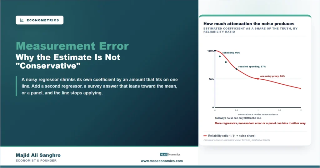
Because the bias is a ratio, it can be tabulated. The relevant quantity is the noise share, the variance of the error relative to the variance of the true regressor, and it converts into a reliability ratio and a percentage shrinkage that hold for any sample size.
| Noise variance relative to true variance | Reliability ratio \( \lambda \) | Estimated coefficient as a share of the truth | What it looks like in practice |
|---|---|---|---|
| 0 | 1.00 | 100% | Administrative records; a variable defined by the researcher |
| 1 to 9 | 0.90 | 90% | Self-reported years of schooling in validated surveys |
| 1 to 4 | 0.80 | 80% | Self-reported annual earnings in many household surveys |
| 1 to 2 | 0.67 | 67% | Recalled expenditure over a long reference period |
| 1 to 1 | 0.50 | 50% | A single noisy proxy for an unobserved concept such as ability |
| 3 to 1 | 0.25 | 25% | The same self-reported variable after first-differencing a two-period panel |

|
|||
The schooling row is the one with the best evidence behind it. Orley Ashenfelter and Alan Krueger, comparing the schooling that identical twins reported for themselves with what their twin reported for them, found reliability ratios for self-reported schooling of about nine tenths, which is to say that a naive regression of wages on reported schooling understates the return by roughly ten percent. The earnings row is where the reflex begins to fail, and the reason is the subject of the next section: earnings errors in surveys are not random noise, and the table’s arithmetic assumes they are.
Why “Conservative” Is the Wrong Word
The classical result holds for one regressor with random error. Three departures from that setting are common, and each one breaks the comforting conclusion that the truth must be larger than the estimate.
The first is a second regressor. When a mismeasured variable shares a regression with correctly measured ones, its own coefficient is still attenuated, but part of the effect it can no longer claim is picked up by whatever correlates with it. Regress wages on noisy schooling and accurately measured experience, and the experience coefficient absorbs some of the schooling effect that the noise released. The bias on the clean variables can be positive or negative, depending on the correlations, and nothing in the data announces which. A researcher who calls the schooling coefficient conservative and the experience coefficient unaffected has it half right and half backwards. The pattern is the same one our article on omitted variable bias describes, because a noisy regressor is, in effect, a partly omitted one.
The second is error that is correlated with the truth. Validation studies that match survey answers to employer or tax records, the work of John Bound, Alan Krueger and their co-authors through the 1990s, found that reported earnings errors are mean-reverting: high earners tend to understate and low earners to overstate. An error that is negatively correlated with the true value compresses the observed variable, and compression is the opposite of the sideways smear in the figure. The observed variance is smaller than the classical formula assumes, the attenuation is weaker than the formula predicts, and in some configurations the coefficient on a mean-reverting variable is overstated rather than understated. Whether an earnings coefficient is biased up or down cannot be settled from the model alone; it depends on how the survey was answered, which is why our article on survey design treats the question wording as part of the econometrics.
The third is a binary regressor. A variable that can only be zero or one cannot have classical error, because the only possible mistakes are flipping a one to a zero or a zero to a one, and those errors are by construction negatively correlated with the truth. Misclassification always attenuates, and it does so more severely than the same amount of noise in a continuous variable; a treatment indicator that is wrong for ten percent of the sample can shrink a treatment effect by well over ten percent. Since the effect of a programme, a policy or a union card is usually estimated with exactly this kind of variable, the attenuation from misreporting participation is one of the most common and least reported biases in evaluation work.
Differencing Makes It Worse
Panel data promises to remove unobserved heterogeneity by comparing each unit with itself, and for the biases it targets it delivers. For measurement error it does the opposite. The within transformation, or first-differencing, subtracts each unit’s own average or own previous value, which removes the persistent part of the true regressor and leaves the transitory part. Measurement error is typically transitory, so it survives the transformation intact while the signal is stripped away. The reliability ratio after differencing is lower than before whenever the true regressor is more persistent than its error, and it is often much lower.
Zvi Griliches and Jerry Hausman set this out in 1986, and the extreme case makes it vivid. If schooling does not change between two survey waves, every bit of within-person variation in reported schooling is error, the reliability ratio of the differenced variable is zero, and the fixed effects estimate of the return to schooling converges to nothing at all. The final row of Table 1 is a milder version of the same arithmetic. This is a large part of why estimates from the panel methods in our article on panel data so often come out smaller than cross-sectional estimates of the same parameter, and it is a reason to be suspicious when a fixed effects result is presented as the careful one without any discussion of what the transformation did to the signal. Griliches and Hausman also showed the way out: because differencing over one period and over several periods attenuates by different, known amounts, comparing the two identifies the error variance and corrects the estimate.
The Repairs, and What Each One Needs
Every correction for attenuation requires information from outside the regression, because the regression itself cannot tell signal from noise. The cleanest source is a second, independent measurement of the same variable. If two reports of schooling have errors that are unrelated to each other, one can serve as an instrument for the other: it is correlated with the true value and uncorrelated with the first report’s error, which is precisely what an instrument has to be. This is the method Ashenfelter and Krueger used with twins, and it is the general form of the instrumental variables repair, with the usual condition that the two errors really are independent, which fails when both reports come from the same respondent with the same misunderstanding.
The second source is a validation study. Where a subsample can be matched to administrative records, the reliability ratio can be estimated directly and the naive coefficient divided by it. The correction is only as good as the assumption that the validation sample’s error structure matches the full sample’s, and it inherits the difficulty that administrative records have errors of their own, though of a different kind. The gap between what a survey says and what the records say is measured in our data article on survey and tax records of top incomes, and it is not small. Where records can replace survey answers rather than validate them, the problem is removed at source, which is one reason administrative data has displaced surveys across so much of applied work.
The third repair is to bound rather than fix. Regressing y on x gives a slope attenuated toward zero; regressing x on y and inverting gives a slope inflated away from it. With one mismeasured regressor and classical error, the truth lies between the two, and reporting both is honest when nothing better is available. Simulation-based corrections that deliberately add further noise, observe how the coefficient shrinks, and extrapolate back to zero noise are the modern version of the same idea. What none of these can do is repair the outcome-side errors that correlate with the regressors, such as rounding that depends on income, and the distinction between a proxy that stands in for a concept and a variable that measures it, which sits at the heart of correlation and causation arguments, is where the classical model stops applying at all. A proxy for ability is not ability with noise added; it is a different variable, and its coefficient answers a different question.
MASEconomics Explains
3 concepts behind errors-in-variables
These concepts are explored in depth across our educational articles library.
Conclusion
Attenuation bias is the one econometric failure whose size can be written on a single line: least squares returns the true coefficient multiplied by the reliability ratio of the regressor, and no amount of data changes that. The line is exact, and it is also narrow. It describes one regressor, measured with random noise, in a cross-section. Add a second regressor and the bias leaks into the clean variables in a direction the data does not reveal. Let the error depend on the truth, as survey earnings errors do, and the shrinkage weakens or reverses. Make the regressor binary and the error can only attenuate, but by more than the noise share suggests. Difference the data to remove fixed effects and the signal goes with them while the noise stays.
The practical rule that follows is to stop describing a noisy estimate as conservative and start asking what is known about the error. Where a second measurement exists, use it as an instrument. Where a validation sample exists, estimate the reliability ratio and report the corrected coefficient beside the naive one. Where a panel estimate is far below its cross-sectional counterpart, say what the transformation did to the signal before crediting the fixed effects with removing bias. And where the variable is a proxy rather than a noisy measurement, say so, because the classical model was never about it. Measurement error is not an excuse for a small coefficient; it is a claim about the data, and claims about the data can be checked.
Frequently Asked Questions
What is attenuation bias?
The tendency of a least squares coefficient to be biased toward zero when the regressor is measured with random error. The estimate converges to the true coefficient multiplied by the reliability ratio, the share of the observed variable’s variance that is signal, so a regressor that is ten percent noise produces a coefficient about ten percent too small regardless of sample size.
Does measurement error in the dependent variable cause bias?
Not if the error is unrelated to the regressors. It joins the disturbance term, leaves the coefficients unbiased and only widens the standard errors. Bias appears when the outcome’s error is correlated with a regressor, for instance when rounding or under-reporting depends on income, and that case has to be handled on its own terms.
Is a coefficient estimated with a noisy regressor always conservative?
Only in the single-regressor case with classical error. With several regressors the bias spreads to the correctly measured variables in either direction. With error that is correlated with the true value, as in self-reported earnings, the attenuation is weaker than the classical formula and the coefficient can even be overstated. The word conservative should be reserved for the case where it has been earned.
Why does fixed effects estimation make measurement error worse?
Because differencing or demeaning removes the persistent part of the true regressor and leaves the transitory part, while measurement error is usually transitory and survives the transformation. The reliability ratio of the transformed variable is lower than that of the original, so the fixed effects estimate is attenuated more severely than the cross-sectional one.
How can attenuation bias be corrected?
With information from outside the regression. A second independent measurement of the same variable can serve as an instrument. A validation sample matched to administrative records gives the reliability ratio directly, and the naive coefficient can be divided by it. Where neither exists, the forward and reverse regressions bound the truth from below and above, and simulation-based corrections extrapolate to zero noise.
What is the reliability ratio?
The variance of the true variable divided by the variance of the observed one, which is the share of what is measured that is signal rather than noise. It lies between zero and one and is the exact factor by which least squares scales the true coefficient under classical error. Validated survey schooling has a reliability ratio around 0.9; a differenced panel variable can fall far lower.
Thanks for reading! The bias fits on one line, and everything people get wrong about it comes from reading that line outside the case it was written for. Happy learning with MASEconomics