In April 2020, the U.S. Treasury sent $1,200 stimulus checks to roughly 160 million Americans. Household spending and saving responses to that transfer remain a central policy question. Two years earlier, Boston’s charter schools produced test score gains that could be attributed to the schools themselves or to student motivation. California’s 1988 tobacco tax reduced smoking, but the counterfactual of what would have happened without the tax is not directly observable. Policy evaluation methods exist to answer this kind of question.
The three workhorses are randomized controlled trials (RCTs), difference‑in‑differences (DiD), and synthetic control. Together they form the toolkit that won the 2021 Nobel Prize in Economic Sciences for David Card, Joshua Angrist, and Guido Imbens, and they now dominate the top journals in economics, public health, and political science.
Each method tackles the same core problem from a different angle. Each has a non‑negotiable assumption that, when violated, makes the results meaningless. Each fits a particular type of policy question better than the others. The choice between them depends on the data available, the policy setting, and the credibility of each assumption.
What Policy Evaluation Is For
For most of the twentieth century, policy evaluation often meant comparing outcomes before and after a program, or comparing people who received the program with those who did not. Both approaches have a fatal flaw. A before-and-after comparison confuses the policy with everything else changing in the economy at the same time. A treated-versus-untreated comparison confuses the policy with whatever made some people sign up in the first place. Job training programs frequently looked ineffective in such studies, not because training failed, but because trainees had been laid off and were on a downward earnings trajectory before the program started.
The “credibility revolution” in empirical economics, documented by Angrist and Pischke (2010), replaced these casual comparisons with a discipline borrowed from clinical trials: every empirical claim must be paired with a credible counterfactual. The counterfactual is the outcome that would have occurred without the policy. It is, by definition, unobservable for any treated unit, since a person, firm, or state experiences either the policy or its absence, never both.
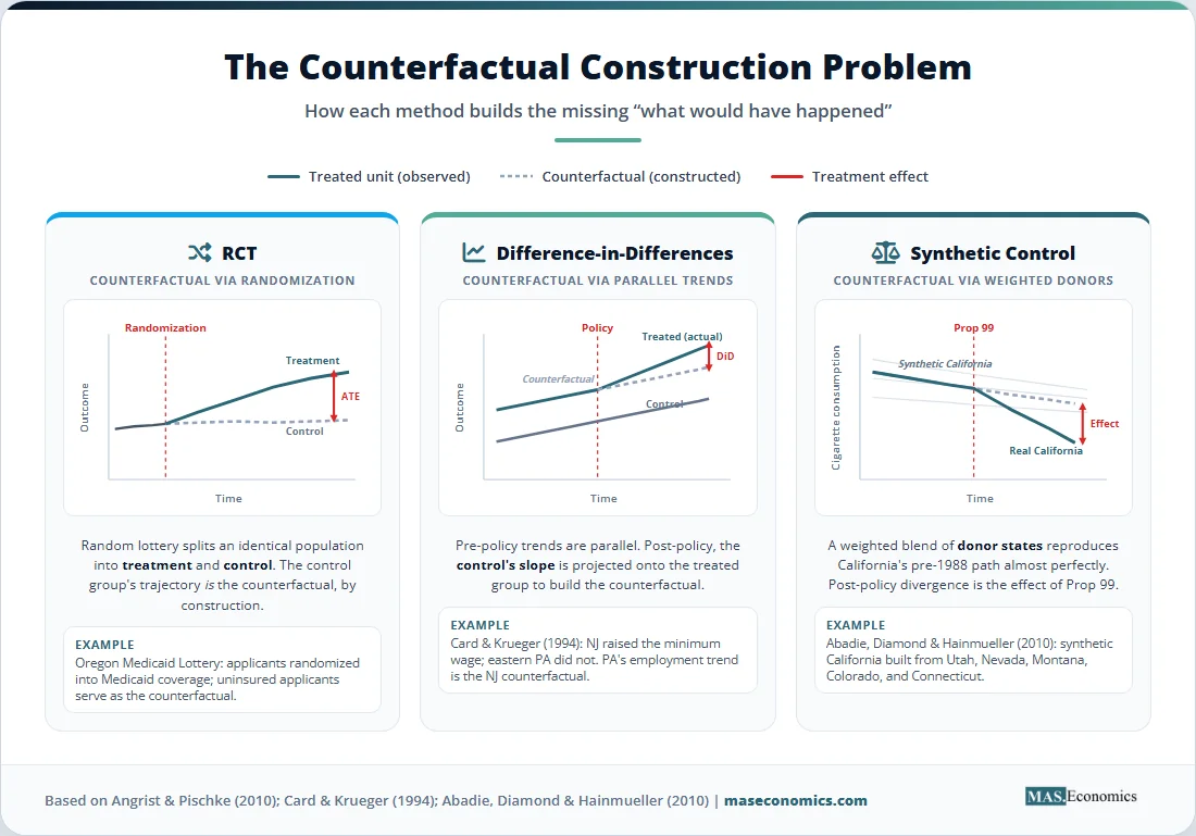
This is the fundamental problem of causal inference. Every modern policy evaluation method is a different strategy for constructing a believable counterfactual. RCTs build it through randomization. DiD builds it from a control group’s trajectory over time. Synthetic control builds it from a weighted average of similar but untreated units. The credibility of the answer depends entirely on whether the chosen counterfactual is plausible.
The stakes are concrete. The U.S. federal government spends roughly $6.8 trillion annually, and the World Bank estimates that more than 30 percent of development aid funds are allocated to programs whose effects are never rigorously measured. When a flagship policy is evaluated badly, governments either kill working programs or scale up failures. When evaluation is done well, the gains compound: deworming children in Kenya, identified through an RCT, became one of the most cost-effective interventions in global health.
RCTs: The Gold Standard
An RCT assigns subjects to a treatment group or a control group by lottery. Random assignment guarantees that, in expectation, the two groups are identical on every characteristic, observable and unobservable. Any difference in outcomes after the intervention can therefore be attributed to the treatment itself. The estimand is the average treatment effect (ATE), the simple difference in mean outcomes between the two groups.
Formally, with \( Y_i(1) \) denoting the outcome under treatment and \( Y_i(0) \) the outcome without, the ATE is:
Random assignment makes the unobserved \( Y_i(0) \) for treated units estimable using the observed average outcome of the control group. No selection bias, no omitted variables, no tricky assumptions about parallel trends.
The track record reads like a tour of modern empirical economics. The Oregon Health Insurance Experiment in 2008 used a state lottery to allocate Medicaid coverage and found large effects on financial security and self-reported health, but no measurable improvement in physical health markers like blood pressure over the first two years. Mexico’s Progresa, randomized across 506 villages in 1997, showed that conditional cash transfers raised school enrollment by 3.4 percentage points for boys and 8 points for girls, evidence that ultimately spread the model to more than 60 countries. The Kenya school deworming trial by Miguel and Kremer (2004) is now textbook material on cost-effective development.
The randomization payoff is real, but RCTs face four practical limits. Cost is the first: large field experiments routinely run into the tens of millions of dollars, and many policy questions cannot be tested at scale on a researcher’s budget. Ethics is the second: a government cannot randomly deny welfare benefits, randomly close hospitals, or randomly bomb cities, no matter how clean the resulting estimate would be. External validity is the third: a deworming RCT in western Kenya does not automatically tell us what deworming will do in urban Bangladesh. The fourth is non-compliance: people assigned to treatment may refuse it, and people assigned to control may find a way to get it. Intent-to-treat analysis preserves the randomization but estimates a diluted effect, while instrumental variables techniques (covered in our IV explainer) can recover the local average treatment effect for compliers.
Most macroeconomic and structural questions also lie permanently outside the reach of RCTs. No one can randomize a financial crisis, a tariff, a recession, or a central bank decision. That is where the quasi-experimental methods come in.
Quasi-Experiments I: Difference-in-Differences
Difference-in-differences turns nature’s accidents into causal evidence. The idea is to compare the change in outcomes for a treated group with the change for an untreated group over the same period. The first difference (treated, before vs. after) absorbs every fixed characteristic of the treated group. The second difference (control, before vs. after) absorbs the common time trend. What remains is the treatment effect.
The simplest two-period DiD estimator is:
where \( T \) and \( C \) index treatment and control groups and 0 and 1 index pre- and post-treatment periods. In a regression framework, the same estimate comes from:
The coefficient \( \tau \) on the interaction term is the DiD estimate. Everything rests on a single identifying assumption: parallel trends. In the absence of treatment, the treated group’s outcome would have evolved on the same trajectory as the control group’s. Graphically, before the intervention, the two lines move in lockstep; after the intervention, the treated line jumps, and the gap is the effect.
The method’s modern profile owes a lot to Card and Krueger (1994), who studied New Jersey’s 1992 minimum wage hike from $4.25 to $5.05 per hour. They surveyed fast-food restaurants in New Jersey and in neighboring eastern Pennsylvania, where the wage stayed flat, both before and after the change. Employment in New Jersey rose slightly relative to the control, contradicting the textbook prediction that minimum wages destroy jobs. The study sparked thirty years of follow-up research and reshaped how economists think about labor markets.
Modern DiD has moved well beyond the two-by-two case. Staggered adoption designs handle settings where different units are treated at different times, such as states legalizing marijuana in different years. Event studies plot the treatment effect period by period, both before and after adoption, allowing direct visual inspection of pre-trends. Recent econometric work by Goodman-Bacon (2021) and de Chaisemartin and D’Haultfoeuille (2020) has shown that the standard two-way fixed effects regression can produce badly biased estimates when treatment effects vary over time, and a wave of new estimators now corrects these problems. Readers who want the full technical picture should see our advanced DiD methods guide.
DiD breaks down when the parallel trends assumption fails. If the treated group was already growing faster than the control before the policy, the estimate captures that pre-existing divergence rather than the treatment. Pre-trend tests, placebo tests on outcomes that should not be affected, and triple-difference designs that subtract out a placebo group are the standard defenses. None of them proves parallel trends; they only fail to reject it.
Quasi-Experiments II: Synthetic Control
Synthetic control was built for a problem DiD handles poorly: a single treated unit with many potential controls and no obvious comparison group. Suppose California passes a tobacco control program in 1988. There is one California, and forty-nine other states with different demographics, smoking cultures, and pre-existing trends. Picking any one of them as the control is arbitrary, and using the unweighted average of the other forty-nine ignores the fact that some states resemble California much more than others.
The method, introduced by Abadie and Gardeazabal (2003) and formalized in Abadie, Diamond, and Hainmueller (2010), constructs a “synthetic California” as a weighted average of other states, with weights chosen so that the synthetic version closely matches the real California on cigarette consumption and predictors of consumption during the pre-treatment period. After 1988, any divergence between actual California and synthetic California is the estimated treatment effect.
The weight vector \( W = (w_1, \dots, w_J)’ \) is chosen to minimize:
subject to \( w_j \geq 0 \) for all \( j \) and \( \sum_j w_j = 1 \). Here \( X_1 \) holds pre-treatment characteristics of California, \( X_0 \) holds the same characteristics for the donor pool, and \( V \) weights the importance of each predictor.
In the California case, the synthetic donor turned out to be a mix of Utah, Nevada, Montana, Colorado, and Connecticut. Per capita cigarette consumption in synthetic California tracked actual California almost perfectly from 1970 through 1988. Then the trajectories split. By the year 2000, real California was smoking 26 fewer packs per capita per year than its synthetic twin, an effect later corroborated by other research designs.
The method shines when the treated unit is unique, the donor pool is large, and the pre-treatment fit is excellent. It has been used to study the economic effects of German reunification, terrorism in the Basque Country, Brexit, and dozens of state-level policy changes. Inference is non-standard: classical standard errors do not apply, and researchers rely on placebo tests that re-run the procedure, assigning treatment to each untreated unit, then compare the actual estimate to the placebo distribution.
The drawbacks are equally specific. Pre-treatment fit can be poor, in which case the synthetic counterfactual is unreliable. The donor pool must contain units that are genuinely comparable. The estimator can be sensitive to the choice of predictors and the period over which fit is optimized. Recent work has produced extensions that address these limits: synthetic difference-in-differences (Arkhangelsky et al., 2021) blends the two approaches, and the generalized synthetic control method handles multiple treated units and interactive fixed effects.
Comparing the Three Approaches
The three methods differ along five dimensions that matter in practice: the kind of data they need, the number of treated units they handle, the assumption that does the identifying work, what they do best, and where they fail. Table 1 lays them out side by side.
| Dimension | Randomized Controlled Trial | Difference-in-Differences | Synthetic Control |
|---|---|---|---|
| Data type | Experimental, researcher-controlled assignment | Observational panel, two or more periods | Observational panel, long pre-treatment window |
| Treated units | Many (often hundreds or thousands) | Many treated and many controls | Typically one or a few treated units |
| Identifying assumption | Random assignment of treatment | Parallel trends in untreated potential outcomes | Good pre-treatment fit and no anticipation |
| Estimand | Average treatment effect (ATE) | Average treatment effect on the treated (ATT) | Treatment effect for the treated unit |
| Strength | Highest internal validity, transparent design | Works at scale on observational data | Disciplined counterfactual for unique events |
| Key limitation | Cost, ethics, external validity, non-compliance | Fails when pre-trends diverge or effects are heterogeneous | Requires good pre-fit and large donor pool |
| Inference | Standard t-tests, randomization inference | Clustered standard errors, event-study tests | Permutation and placebo tests |
| Classic example | Oregon Medicaid lottery (2008) | Card and Krueger minimum wage (1994) | California Proposition 99 tobacco (2010) |

|
|||
Two patterns stand out. First, RCTs win on credibility but lose on coverage. They produce the cleanest estimates, but only for questions a researcher can actually randomize. Second, the two quasi-experimental methods are not redundant. DiD scales: it can absorb thousands of treated units and produce a single average effect. Synthetic control specializes: it gives a transparent counterfactual when the question is about a single state, country, or firm. A researcher asking “what did this one policy do to this one place?” will reach for synthetic control. A researcher asking “what does this kind of policy do on average?” will reach for DiD or an RCT.
When to Use Which Method
The choice flows from the structure of the problem, not from methodological preference. Three questions narrow the options quickly.
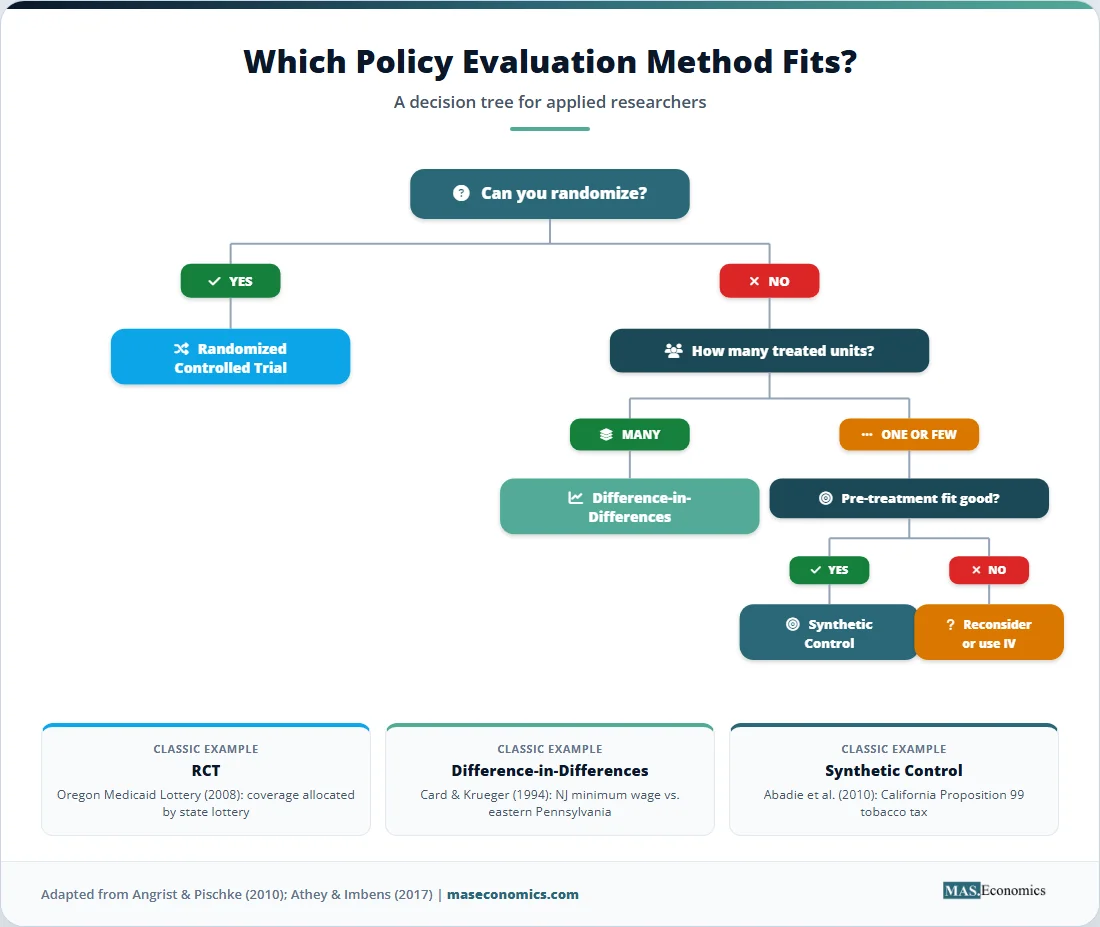
The first question is whether random assignment is feasible and ethical. If a government, NGO, or firm can randomize the treatment to a large pool of subjects, an RCT is almost always the right answer. The estimate is unbiased by construction, the design is easy to communicate to non-economists, and the result is replicable. J-PAL, IPA, and the World Bank’s DIME unit have built infrastructure that makes this option more feasible than it was twenty years ago.
The second question, when randomization is off the table, is how many units actually receive the treatment. If many states, firms, schools, or workers are treated at staggered dates, modern DiD methods are the natural fit. If a single high-profile unit is treated, such as one country leaving the EU or one state changing a tax code, synthetic control or its modern variants are the right starting point. The intuition is mechanical: DiD averages across many treated units to wash out idiosyncratic shocks, while synthetic control concentrates on a single trajectory.
The third question is whether the data support the identifying assumption. For DiD, this means checking pre-trends, running placebo tests on outcomes that should be unaffected, and considering whether anticipation effects could distort the estimate. For synthetic control, it means examining the pre-treatment fit and the composition of the donor pool. For RCTs, it means checking the balance across treatment and control on observable characteristics and tracking compliance. None of these checks proves the assumption holds, but they expose obvious failures.
| If the question is… | And the data look like… | The right tool is… |
|---|---|---|
| Effect of a small-scale program on individuals | Researcher controls assignment | RCT |
| Effect of a state-level policy across many states | Panel of states, staggered adoption | Staggered DiD or event study |
| Effect of a single high-profile policy on one unit | One treated unit, large donor pool | Synthetic control |
| Effect with both spatial and temporal variation | Few treated units, structured panel | Synthetic DiD |
| Effect when an instrument is available | Cross-section with valid IV | Instrumental variables |
|
|
||
The methods are best understood as complements, not substitutes. The current standard in top-tier policy research is to lead with one method and then check whether alternatives produce similar answers. Athey and Imbens (2017) argue that triangulation across designs is the closest empirical economics gets to a proof of robustness. When an RCT, a DiD analysis, and a synthetic control study converge on similar magnitudes, the policy effect is real. When they diverge, the divergence itself is informative about which assumptions are biting.
Estimates Across Methods
The figure below illustrates how estimates of the same policy effect can differ across methods, using a stylized version of the California tobacco control case. Each method produces a per-capita reduction in cigarette consumption a decade after the 1988 program, with synthetic control providing the headline estimate of roughly 26 packs, a comparable-states DiD producing 18 packs, and an early-period RCT-style intervention on smoking cessation programs in clinics yielding effects in the 8 to 12 pack range. The chart makes the practical point: methods that look at different counterfactuals can produce different magnitudes, and each magnitude answers a slightly different question.
Figure 1. Estimated reduction in per-capita cigarette consumption (packs per year, ten-year horizon) across three policy evaluation methods, California tobacco control case. Sources: Abadie, Diamond, and Hainmueller (2010); supplementary state-level DiD analyses; clinical smoking cessation RCT meta-analyses.
Common Pitfalls in Policy Evaluation
No method survives sloppy application. RCTs lose their edge when compliance is low, attrition is differential between arms, or the experimental population is too narrow to generalize. The Oregon Medicaid lottery, for all its design strength, applied to a specific group of low-income adults in one state during one period, and its findings on health outcomes do not automatically extend to children or to a national Medicaid expansion.
DiD fails most often through pre-trend violations and treatment effect heterogeneity. The Goodman-Bacon decomposition revealed that two-way fixed effects regressions in staggered settings can place negative weights on some comparisons, occasionally flipping the sign of the estimate. Modern DiD estimators by Callaway and Sant’Anna (2021), Sun and Abraham (2021), and de Chaisemartin and D’Haultfoeuille handle this, but they require deliberate choice rather than the default regression.
Synthetic control fails when the pre-treatment fit is poor, when no convex combination of donors can reproduce the treated unit’s trajectory, or when the donor pool itself was affected by spillovers from the treatment. The method also assumes no anticipation: if the treated unit changed behavior in advance of the policy, the pre-treatment fit is contaminated, and the post-treatment gap is mismeasured. Robustness checks that drop individual donors, vary the predictors, and examine in-time placebos are now expected in any serious application.
External validity binds all three. An effect estimated for one population, period, or context is not guaranteed to transfer. The replication crisis in social science taught economists that even well-identified estimates can be fragile across settings. The sober response is to design evaluations that measure mechanisms, not just average effects, and to combine several studies through meta-analysis or structural extrapolation. Natural experiments, when handled with the same care as designed experiments, contribute to this evidence base, as do the broader research designs covered in our research methods primer.
MASEconomics Explains
4 economic concepts behind policy evaluation methods
Conclusion
Policy evaluation methods have moved from comparing means to constructing credible counterfactuals, and the three workhorses each occupy a clear niche. RCTs deliver the cleanest internal validity at the cost of feasibility. Difference-in-differences scales to large policy questions when parallel trends hold, and pre-trends are flat. Synthetic control specializes in single high-profile interventions where one unit needs a tailored counterfactual. The choice between them is dictated by the structure of the question, the data available, and the assumptions a researcher is willing to defend. Triangulating across methods has become standard practice in the top journals, and convergence across designs now carries more weight than any single estimate.
Did you find this article helpful? Share it with someone who loves economics. And remember, at MASEconomics, we make complex ideas simple.