Producer Equilibrium: Where Isoquant Meets Isocost

A firm committed to producing 10,000 units faces countless input combinations that can do the job, from a heavily automated setup with few workers to a labor-intensive one with little machinery. Only one of those combinations costs the least. Producer equilibrium is that least-cost point, the input mix where the firm cannot rearrange capital and labor to produce the same output for less money. It is the moment the technology described by the isoquant and the prices described by the isocost line resolve into a single decision.

The point sits at the intersection of the two halves of production theory. The isoquant comes from the analysis of production functions and isoquant curves and shows what input bundles yield a target output. The isocost line shows what bundles a given budget can buy. Producer equilibrium is where the lowest affordable isocost line just touches the required isoquant, and that tangency is the foundation of cost-minimizing behavior studied throughout the costs of production.

Equilibrium Sits at the Tangency Point

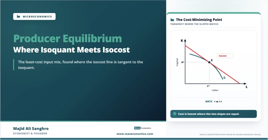
Producer equilibrium occurs where an isocost line is tangent to the isoquant for the target output. Graphically, the firm wants the lowest possible isocost line, the one closest to the origin, that still reaches the required isoquant. A line closer to the origin represents less spending but fails to touch the isoquant, so it cannot produce the output. A line farther out reaches the isoquant but costs more than necessary. The tangent line is the unique lowest-cost line that meets the output target.

The diagram shows why the tangency is special. The red isocost line touches the isoquant at exactly one point, E, and lies below it everywhere else, which marks it as the cheapest line that still reaches the output. The grey dashed line represents a smaller budget; it stays below the isoquant at every point and never reaches it, so that outlay cannot produce the target. At E, the firm buys K* units of capital and L* units of labor, the combination that produces output Q at the minimum possible cost.

Tangency Equates Two Slopes

The economic meaning of the tangency lies in the slopes. At the point of tangency, the slope of the isoquant equals the slope of the isocost line. The slope of the isoquant is the marginal rate of technical substitution, the rate at which the technology lets capital be traded for labor while holding output constant. The slope of the isocost line is the wage-rental ratio, the rate at which the market lets capital be traded for labor at constant cost. Equilibrium is where these two rates coincide.

Producer Equilibrium Condition

At equilibrium the marginal rate of technical substitution equals the wage-rental ratio, so the ratio of marginal products equals the ratio of input prices.

Rearranging the condition reveals the deeper logic. Setting the ratio of marginal products equal to the ratio of prices is the same as setting the marginal product per dollar equal across inputs. The last dollar spent on labor adds exactly as much output as the last dollar spent on capital. If that were not true, the firm could shift a dollar from the lower-yield input to the higher-yield one and produce more for the same cost, which means it was not yet at the minimum. Equality of the marginal product per dollar is the signature of a genuine cost-minimizing point.

Equal Marginal Product per Dollar

Cost minimization requires that the marginal product of the last dollar spent on each input be equal, leaving no profitable reallocation between inputs.

Equilibrium as a Constrained Optimization

The tangency result is the graphical face of a formal optimization. The firm minimizes total cost subject to the constraint that output equals the target, a problem solved with the method of Lagrange multipliers covered in the study of optimization techniques in economics. Setting up the Lagrangian for cost minimization and taking first-order conditions reproduces exactly the tangency condition derived geometrically.

The first-order conditions require the ratio of each input’s marginal product to its price to equal a common value, the Lagrange multiplier, which carries an economic interpretation as the marginal cost of producing one more unit of output. The geometry and the calculus agree completely: the point where the isoquant and isocost line are tangent is the point where the Lagrangian conditions hold. The diagram is the picture, the Lagrangian is the proof, and both identify the same input mix as the cost-minimizing choice.

Table 1. Reading Points Relative to Producer Equilibrium

Situation	Slope comparison	What the firm should do
MRTS greater than w/r	Isoquant steeper than isocost	Use more labor, less capital
MRTS less than w/r	Isoquant flatter than isocost	Use more capital, less labor
MRTS equals w/r	Slopes equal at tangency	Stay; cost is minimized
Source: MASEconomics editorial synthesis of standard producer theory.

The table reads the diagram as a decision rule. Where the isoquant is steeper than the isocost line, the technology values labor more highly than the market charges for it, so substituting toward labor lowers cost. Where the isoquant is flatter, the reverse holds and the firm substitutes toward capital. Only where the two slopes match is no further substitution profitable, which is the defining property of producer equilibrium.

Equilibrium Holds Output and Prices Fixed

Producer equilibrium answers one specific question: for a given output and given input prices, what is the cheapest input mix. It does not determine how much output the firm should produce, which depends on demand and the price of the product, nor does it explain how the firm responds when it scales production up or down. Tracing equilibrium across different output levels generates the expansion path, a separate construction that connects the tangency points.

The result also assumes the convex, smooth isoquants of the standard case. When inputs are perfect substitutes, the least-cost choice is a corner solution using only the cheaper input, and there is no interior tangency. When inputs are perfect complements, the equilibrium sits at the corner of the L-shaped isoquant, again without a smooth tangency. Within the standard case, producer equilibrium is the precise statement of cost-minimizing input choice, and it is the building block on which the firm’s cost curves and supply behavior are built.

Explains

Conclusion

The producer equilibrium is the cost-minimizing input combination, located where the lowest affordable isocost line is tangent to the isoquant for the target output. At that point, the firm buys the specific quantities of capital and labor that produce the required output for the least total cost, with no rearrangement of inputs able to lower the bill further.

The tangency carries a precise economic condition: the marginal rate of technical substitution equals the wage-rental ratio, which is equivalent to equating the marginal product per dollar across inputs. The technology’s rate of trade-off between inputs matches the market’s rate, so the last dollar spent on labor yields the same extra output as the last dollar spent on capital. The same condition emerges from the formal cost-minimization problem solved with Lagrange multipliers, so the graphical and algebraic accounts agree.

The result is bounded by its assumptions. It holds output and input prices fixed and applies to the standard case of smooth, convex isoquants, giving way to corner solutions for perfect substitutes and complements. Within that scope, producer equilibrium converts the technology of the isoquant and the prices of the isocost line into a single determinate input choice, and that choice is the basis for the firm’s cost curves and its position in the wider theory of supply.

Frequently Asked Questions

Thanks for reading! If you found this helpful, share it with friends and spread the knowledge. Happy learning with MASEconomics