Regression Discontinuity Design: Estimating Causal Effects at a Cutoff

A scholarship rule, pension age, test-score cutoff, income threshold, or electoral margin can place two people on opposite sides of a policy line even when they are nearly identical in every other observable way. Regression discontinuity design uses that sharp policy line to estimate a causal effect by comparing units just below and just above the cutoff.

The basic idea is local comparison. A student who scores 79.9 and misses a scholarship is likely to be more comparable to a student who scores 80.1 and receives it than to a student who scores 50 or 100. A firm just below an eligibility threshold may resemble a firm just above it. A district where a party barely loses an election may resemble a district where it barely wins. When treatment changes discontinuously at the threshold, but other determinants of the outcome change smoothly, the jump in the outcome can be interpreted as a causal effect near the cutoff.

Regression discontinuity design, often abbreviated as RDD or RD, is one of the most important quasi-experimental tools in applied economics. It does not require random assignment across an entire population. Instead, it asks whether assignment around a threshold is as good as random. That makes it powerful, but also narrow. RDD can produce credible local causal evidence, but only when the cutoff is real, the running variable is measured correctly, and units cannot precisely manipulate their position around the threshold.

Cutoff as a Local Experiment

RDD starts with a rule. Treatment is assigned by whether a running variable crosses a known cutoff. The running variable may be a test score, age, vote share, income, population size, pollution reading, credit score, or any measurable index used by an institution to decide eligibility. The cutoff is the point where assignment changes.

Suppose a government training program is offered to workers whose unemployment-risk score is at least 60. Workers with scores of 59.8 and 60.2 are not randomly chosen from the full population, but they may be similar around the cutoff. If the probability of receiving training jumps at 60, and no other factor jumps at exactly 60, then any discontinuous change in later earnings at that score can be attributed to the program for workers near the threshold.

This is why RDD belongs inside causal inference, not only regression modeling. The key claim is not that a line can be fitted on a scatter plot. The key claim is that the treatment rule produces a credible comparison at the boundary. The regression is a tool for estimating the jump. The research design is the reason the jump can be read causally.

The method has a long history, beginning with Donald Thistlethwaite and Donald Campbell’s 1960 evaluation work. It became especially influential in economics after later methodological development and applied use. Lee and Lemieux’s “Regression Discontinuity Designs in Economics” describes why economists treat RD as a quasi-experimental design and how its validity depends on incentives, estimation choices, and the interpretation of local effects.

Role of the Running Variable

The running variable is the variable that determines treatment assignment. It is sometimes called the forcing variable or assignment variable. It must be observed, ordered, and linked directly to the eligibility rule. Without a clear running variable, there is no regression discontinuity design.

A clean RDD has three core pieces: a running variable \(X_i\), a cutoff \(c\), and a treatment indicator \(D_i\). In a sharp RDD, treatment switches from 0 to 1 exactly at the cutoff:

Sharp RD Assignment Rule:

Treatment is assigned when the running variable reaches or exceeds the cutoff.

The outcome \(Y_i\) may be earnings, employment, test performance, firm growth, health use, pollution exposure, voting behavior, or another policy-relevant variable. The RD estimand is the size of the discontinuity in the conditional expectation of the outcome at the cutoff:

Local Treatment Effect at the Cutoff

The effect is local because it compares units just above and just below the threshold.

This notation clarifies the central logic. RDD does not compare all treated units with all untreated units. It compares the two sides of the cutoff in the limit as observations approach the threshold. That local nature gives RD its credibility and its limitation at the same time.

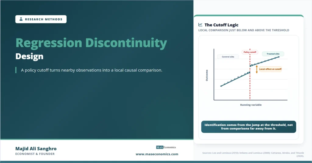
Visualizing the RD Cutoff

The most useful first diagnostic in an RDD study is visual. The researcher plots the outcome against the running variable, marks the cutoff, and checks whether the fitted relationship shows a visible jump at the threshold. The graph does not prove identification, but it helps readers see the design.

The vertical line marks the cutoff. The fitted relationship can slope on both sides because the running variable may affect the outcome. The identifying information is the discontinuous jump at the threshold, not the general slope of the line. If the outcome changes smoothly through the cutoff, there is no visible RD effect. If the outcome jumps precisely where eligibility changes, the graph supports the design’s central claim.

Sharp vs Fuzzy RD

The sharp RD case is conceptually clean: crossing the cutoff fully determines treatment. Everyone below is untreated, and everyone above is treated. Many real policies are not that exact. A cutoff may change the probability of treatment without determining treatment perfectly. This is called fuzzy RD.

Consider a school-support program where students below a test-score threshold become eligible for tutoring, but not every eligible student attends. The cutoff creates a jump in the probability of receiving tutoring, but treatment take-up is incomplete. The outcome may also jump at the cutoff. In that case, the fuzzy RD estimand scales the outcome jump by the treatment-probability jump.

Fuzzy RD Wald Ratio

The numerator is the outcome jump. The denominator is the treatment take-up jump.

The fuzzy design is closely related to instrumental variables. Crossing the cutoff acts like an instrument for actual treatment. The estimate applies to compliers near the cutoff, meaning units whose treatment status changes because they crossed the threshold. This is not necessarily the average effect for all units or all treated units.

Table 1. Main Regression Discontinuity Specifications

Design type	Assignment rule	Estimated effect	Main credibility question
Sharp RD	Treatment changes from 0 to 1 at the cutoff	Local average effect at the threshold	Are units just below and just above comparable?
Fuzzy RD	Treatment probability jumps at the cutoff	Local effect for compliers near the threshold	Does the cutoff strongly change treatment take-up?
Local linear RD	Fit separate local lines on each side	Jump in fitted outcomes at the cutoff	Is the chosen bandwidth credible?
RD with covariates	Include predetermined covariates for precision	Conditional local effect at the cutoff	Are covariates smooth through the cutoff?
Discrete-score RD	Running variable has limited support points	Approximate local effect around threshold bins	Is there enough variation close to the cutoff?
Source: MASEconomics synthesis based on Lee and Lemieux (2010), Imbens and Lemieux (2008), and Cattaneo, Idrobo, and Titiunik (2020).

Continuity as the Causal Basis

The core identifying assumption in RDD is continuity. In plain language, all determinants of the outcome other than treatment should move smoothly through the cutoff. If potential outcomes would have been continuous at the threshold without treatment, then a discontinuity in observed outcomes can be attributed to treatment.

This assumption is not the same as saying treated and untreated units are identical everywhere. It says that units extremely close to the cutoff are comparable. A household barely eligible for a benefit and a household barely ineligible may differ in treatment status because of the rule, not because of a bigger economic difference. Far from the cutoff, that logic weakens.

Continuity links RDD to internal validity. The design is internally credible when the cutoff creates a clean local comparison. It is less credible if the threshold coincides with other institutional changes, if the running variable is manipulated, or if units sort strategically around the boundary.

Manipulation at the Cutoff

RDD becomes weak when people, firms, schools, or governments can precisely control which side of the cutoff they land on. If the cutoff is a test score and teachers can adjust borderline scores, students just above the threshold may differ systematically from students just below it. If a firm can report revenue just below a tax threshold, the density of firms may bunch on one side. If a city can manipulate population figures to qualify for grants, the threshold no longer behaves like a local experiment.

Researchers therefore check whether the running variable itself changes suspiciously at the cutoff. A visible pile-up just above or below the threshold can indicate sorting. They also test whether predetermined covariates, such as age, prior earnings, past test scores, or baseline firm size, remain balanced around the cutoff. These covariates should not jump at the same point as treatment.

The logic is similar to concerns in natural experiments. A policy rule can create useful variation, but only if the rule does not also create systematic selection that contaminates the comparison. The closer the assignment process is to a mechanical threshold that agents cannot finely manipulate, the stronger the RD design becomes.

Bandwidth Selection

The bandwidth defines how close observations must be to the cutoff to enter the analysis. A narrow bandwidth compares units very close to the threshold, improving comparability but reducing sample size. A wide bandwidth uses more data, improving precision but increasing the risk that the two sides are no longer comparable.

This trade-off makes bandwidth selection one of the most important choices in RDD. If the bandwidth is too wide, the estimate may reflect functional-form assumptions rather than a local discontinuity. If it is too narrow, the estimate may be noisy and imprecise. Imbens and Lemieux’s “Regression Discontinuity Designs: A Guide to Practice” helped establish many practical concerns around implementation, including bandwidth choice, specification, and graphical analysis.

A credible RD paper usually reports more than one bandwidth. The preferred estimate should be justified, and alternative bandwidths should show whether the result is stable. This is not p-hacking when the preferred rule is transparent and sensitivity checks are reported honestly. It becomes a credibility problem when the published bandwidth appears chosen because it produces the desired result.

Bandwidth also interacts with statistical power. An RD design may be credible but underpowered if few observations lie close to the cutoff. That is why sample size planning matters before a study relies on a threshold design. A policy cutoff with too few near-threshold observations may produce estimates that are too noisy to guide policy.

Functional Form Considerations

A common mistake in RD analysis is to fit a complicated global polynomial across the whole data range and treat the estimated threshold jump as causal. The danger is that the model’s curvature, not the data near the cutoff, may create the apparent discontinuity. Modern RD practice usually favors local estimation near the cutoff, often using local linear regression with separate slopes on each side.

The reason is conceptual. RDD is a local design. The outcome relationship far from the cutoff should not dominate the estimated effect at the boundary. A flexible curve that fits distant observations well may behave badly near the threshold. A simple local comparison often matches the design logic better than an impressive-looking global fit.

This is where the relationship between RDD and simple regression can be misleading. In ordinary regression, the full sample helps estimate a conditional association. In RDD, observations closest to the cutoff usually carry the most identification value. Regression is used, but the design does not depend on believing that one global line describes the entire relationship.

Local Policy Interpretation

The local nature of RDD is not a weakness by itself. Many policy questions are genuinely local. A university may want to know whether admitting students just above an entrance cutoff changes graduation outcomes. A government may want to know whether firms just eligible for a subsidy grow faster than firms just ineligible. A regulator may want to know whether crossing a pollution threshold changes compliance behavior.

In these cases, the cutoff population may be exactly the policy-relevant group. Threshold rules often determine who gets scarce resources, who qualifies for support, who faces regulation, or who receives a different institutional treatment. An RD estimate can be especially useful when the policy debate concerns the marginal units around the boundary.

The problem begins when a local estimate is overstated. A scholarship effect for students near the eligibility threshold may not apply to students far below or far above it. A credit-policy effect for borrowers near a score cutoff may not apply to all borrowers. A close-election RD estimate may describe competitive districts, not landslide districts. Policy evaluation requires both credible identification and careful interpretation of whose effect is being measured.

Close Elections, Test Scores, and Eligibility Rules

Economists use RDD when institutions assign treatment through thresholds. Close elections are a classic example. A candidate who wins with 50.1 percent of the vote may be compared with a candidate who loses with 49.9 percent. If districts near the 50 percent cutoff are comparable, the jump in later outcomes can identify the effect of holding office for close races.

Education research often uses score cutoffs. Students may enter gifted programs, remedial tracks, scholarships, or selective schools based on a test-score threshold. Labor and social-policy research uses income, age, unemployment duration, disability ratings, or poverty-score cutoffs. Public finance and regulation studies use firm-size thresholds, population thresholds, revenue thresholds, or environmental measures.

Each setting requires institutional knowledge. The researcher must understand how the cutoff is applied, whether exceptions exist, whether agents know the rule in advance, and whether crossing the threshold changes only one treatment or several policies at once. A clean graph cannot substitute for understanding the assignment rule.

Threats to RD Validity

A good RD paper usually addresses several threats. The first is manipulation of the running variable. The second is covariate imbalance. The third is multiple policies changing at the same cutoff. The fourth is limited data near the threshold. The fifth is sensitivity to bandwidth and functional form.

Another threat is measurement error in the running variable. If the assignment score is recorded incorrectly, or if the researcher observes a proxy rather than the true eligibility variable, the cutoff may be blurred. In fuzzy RD, treatment take-up may be weak. If crossing the threshold barely changes treatment probability, the design may have little identifying power.

There is also a communication problem. RD graphs can look persuasive even when the assumptions are weak. Readers should ask whether the discontinuity is visible, whether the treatment rule is institutional rather than invented after the fact, whether the cutoff was known in advance, and whether the effect remains stable under reasonable alternative choices. These checks connect RD to broader concerns about pre-analysis plans and transparent research design.

RDD vs Other Evaluation Designs

RDD sits between randomized experiments and observational regression. It does not randomize treatment in the broad experimental sense, but it can approximate random assignment locally when the cutoff is credible. It is usually stronger than a simple treated-versus-untreated comparison because treatment assignment follows a known rule. It is narrower than a randomized controlled trial because the estimate applies around the threshold.

Compared with difference-in-differences, RD relies on a discontinuity in the running variable rather than parallel trends over time. Compared with matching, it does not require selecting comparison units based on many observed characteristics. Compared with instrumental variables, fuzzy RD uses the cutoff as an instrument, but only locally. Compared with ordinary multiple regression, RD places far more weight on the institutional assignment rule.

This is why RDD is best understood as a design before it is understood as an estimator. The method asks whether a threshold rule generates credible local variation. Once that design question is answered, regression tools estimate the size of the discontinuity.

Explains

Conclusion

Regression discontinuity design is powerful because it turns a policy cutoff into a local comparison. When units just below and just above a threshold are comparable, and treatment changes discontinuously at that threshold, the jump in outcomes can estimate a causal effect. The design is especially useful in economics because many real institutions use eligibility rules, scores, ages, vote shares, income thresholds, and population cutoffs to assign policy treatment.

The strength of RDD is also its boundary. It estimates an effect near the cutoff, not automatically for the whole population. Its credibility depends on continuity, limited manipulation, enough observations near the threshold, and transparent choices about bandwidth and functional form. A convincing RD study shows the assignment rule, graphs the discontinuity, checks for sorting, tests covariate balance, and reports sensitivity to reasonable specifications.

RDD is not just a regression with a threshold variable. It is a research design built on institutional rules. When the rule is real, and the local comparison is credible, RD can provide some of the clearest nonexperimental evidence in applied economics. When the cutoff is manipulated, weak, or poorly understood, the same design can mislead. The difference lies in the credibility of the threshold.

Frequently Asked Questions

Thanks for reading! If you found this helpful, share it with friends and spread the knowledge. Happy learning with MASEconomics