For most of the post-war period, recession and inflation were treated by economists as opposite problems. Demand was either too strong, producing inflation, or too weak, producing recession and unemployment. The standard policy response followed mechanically from the diagnosis: tighten when demand was hot, ease when it was cold. The early 1970s broke that framework. Between 1973 and 1975, the United States simultaneously experienced a doubling of inflation from roughly 6 to 12 percent and a recession that pushed unemployment from 4.6 to 9 percent. The combination was so unfamiliar that a new word had to be coined for it. Stagflation explained the puzzle that the textbook trade-off could not: an economy in which prices were accelerating, and output was falling at the same time. Half a century later, the term has returned, first in the 2022 inflation surge that arrived alongside slowing growth in much of Europe, and again in 2026 as the Iran-Hormuz oil shock combined with a cooling US labour market.
Definition and Distinctiveness of Stagflation
Stagflation is the simultaneous occurrence of high inflation and stagnant or contracting economic output, typically accompanied by rising unemployment. The word itself was first used in 1965 by the British politician Iain Macleod in a speech to the House of Commons, describing the combination of stagnation and inflation as “a stagflation situation”. It entered the economics literature properly during the 1970s, when the phenomenon it described became unmistakable in the data of every major advanced economy.
What makes stagflation analytically unusual is that it appears to violate the standard textbook relationship between inflation and unemployment. Under conventional demand-side reasoning, an economy operating below capacity should experience disinflation as firms cut prices and workers accept lower wages to maintain employment. An economy operating above capacity should experience inflation as scarce labour and goods bid prices up. Inflation and unemployment should move in opposite directions, tracing out the negatively sloped relationship that A.W. Phillips identified in UK data from 1861 to 1957. The 1970s showed that this relationship was not a structural feature of the economy but a contingent statistical regularity that could and did break down.
The breakdown happens because the Phillips curve, as originally formulated, assumes that inflation is driven by demand pressure relative to potential output. When inflation arises from a different source, from a sudden contraction in the supply of an essential input such as oil, food, or labour, the curve no longer applies. A negative supply shock raises prices and reduces output at the same time, because firms face higher input costs and must either pass them through (raising prices) or absorb them (reducing output and employment). In either case, the standard inverse relationship between inflation and unemployment is replaced by a positive co-movement.
Aggregate Supply and Demand Mechanics of Stagflation
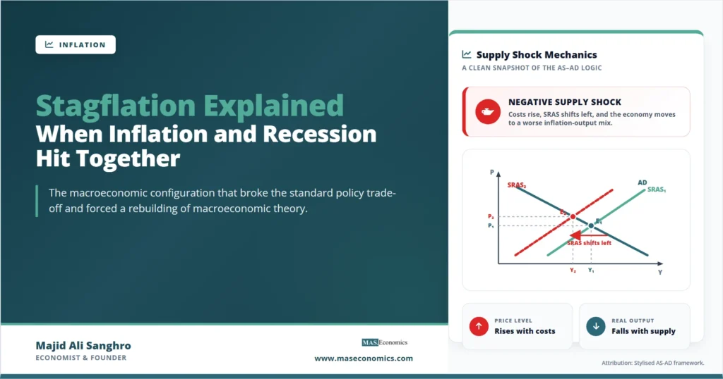
The clearest way to understand stagflation is through the aggregate supply curve. A negative supply shock shifts the short-run aggregate supply curve leftward, raising the price level and reducing real output simultaneously. The shock can come from any source that raises the cost of producing goods and services across the economy: an oil price quadrupling, a collapse in agricultural output, a sudden tightening of labour supply, or a major disruption to global supply chains. The mechanism is the same in each case.

The diagram makes the central asymmetry visible. A demand shock moves the price level and output in the same direction, so the policy diagnosis is clear: stimulate when both fall, tighten when both rise. A supply shock moves them in opposite directions, so any policy that addresses one problem worsens the other. Tightening monetary policy to reduce inflation deepens the recession. Easing monetary policy to support output adds to inflation. There is no choice that delivers both objectives. This is the genuine policy bind that stagflation creates, and it is why central banks treat sustained negative supply shocks as the hardest macroeconomic environment to manage.
The Failure of the Phillips Curve
The Phillips curve, in its original 1958 formulation, was an empirical regularity. Phillips plotted UK wage inflation against unemployment for nearly a century of data and found a stable negative relationship. The natural interpretation was that policymakers could choose a point on the curve: accept higher inflation to deliver lower unemployment, or accept higher unemployment to deliver lower inflation. The 1960s in the United States and the United Kingdom were dominated by this view, and policy was set as if the trade-off were exploitable.
The trade-off broke in the 1970s for the reason that Milton Friedman and Edmund Phelps had predicted in 1967 and 1968. The empirical Phillips curve held only as long as inflation expectations remained anchored. Once households and firms began to expect higher inflation in the future, they built it into wage negotiations and pricing decisions, shifting the short-run curve upward. The result was that any given level of unemployment was associated with progressively higher inflation. The economy moved not along the Phillips curve but along a sequence of curves, each shifted by changing expectations. In a stagflation, the curve appears to slope the wrong way because the underlying source of the inflation is supply rather than demand.
The intellectual consequence was the displacement of the static Phillips curve by the expectations-augmented version, which holds that the trade-off exists only in the short run and only when inflation expectations are anchored. The Phillips curve relationship survives in modified form in modern macroeconomics, but it no longer carries the weight of a policy menu. The lesson from the 1970s is that any inflation-unemployment combination is achievable in the short run, but only one combination is sustainable in the long run, and it is the one consistent with the natural rate of unemployment.
The 1970s Oil‑Shock Stagflation
The 1970s stagflation in the United States, the United Kingdom, and most of continental Europe was driven by two large oil price shocks, in 1973 and 1979, layered on top of a domestic policy environment that was already pushing inflation higher. The October 1973 OPEC embargo, prompted by Western support for Israel in the Yom Kippur War, quadrupled the price of crude oil from around $3 per barrel to over $12 within months. The 1979 Iranian Revolution and subsequent disruptions to Iranian oil production roughly doubled prices again, reaching nearly $40 per barrel by 1980.
The macroeconomic consequences were severe. In the United States, inflation rose from 3.2 percent in 1972 to 11.0 percent in 1974, fell back to 5.7 percent in 1976, then climbed again to 13.5 percent by 1980. Unemployment rose from 4.9 percent in 1973 to 8.5 percent in 1975 and stayed elevated for most of the decade. Real GDP contracted in five of the ten years from 1970 to 1980. Living standards stagnated for the median worker for the first time since the war.
The episode was not purely a supply shock. Loose monetary policy under Federal Reserve Chair Arthur Burns, fiscal expansion to fund the Vietnam War and Great Society programmes, and the abandonment of the Bretton Woods exchange rate system in 1971 all contributed. But the oil shocks were the proximate cause that turned an inflation problem into stagflation. The disinflation that ended the episode required the Volcker tightening from 1979 onward, with the federal funds rate reaching 20 percent in 1981 and a deep recession that pushed unemployment to 10.8 percent in 1982. By 1983, inflation was back below 4 percent, and a long expansion began. The cost of breaking entrenched inflation expectations was the deepest recession since the 1930s. Cross-country comparison shows that the same dynamics played out, with national variation, across Western Europe and Japan.
The 2022 Supply‑Shock Stagflation
The 2022 inflation surge in advanced economies revived the term stagflation in policy discussion for the first time in a generation. Inflation rose from around 2 percent at the start of 2021 to peaks of 9.1 percent in the United States (June 2022), 11.1 percent in the United Kingdom (October 2022), and 10.6 percent in the eurozone (October 2022). The drivers were a combination of pandemic-era supply chain disruptions, post-lockdown demand shifts, and the energy and food price shock triggered by the Russian invasion of Ukraine in February 2022. The 2022 energy shock bore strong structural similarities to 1973: a sudden contraction in the supply of an essential input, transmitted through every cost-sensitive sector of the economy.
The episode qualified as stagflation in Europe but not, on a strict reading, in the United States. Eurozone GDP growth fell sharply through 2022, reaching near-zero by the fourth quarter, while inflation peaked in double digits. The UK entered a technical recession in late 2023 with inflation still above target. In the United States, however, the labour market remained tight throughout the disinflation, with unemployment staying near 50-year lows even as inflation climbed and then fell. The US experience was therefore a high-inflation episode with resilient growth, closer to an inflation surge than a textbook stagflation.
The policy response across all three economies was almost entirely monetary. The Federal Reserve raised rates by 525 basis points between March 2022 and July 2023. The ECB raised rates by 450 basis points. The Bank of England raised the Bank Rate from 0.1 to 5.25 percent. Fiscal policy did not contract; in many countries, it expanded to cushion households from the energy price shock. The disinflation that followed was relatively rapid and relatively painless by historical standards, with US inflation falling from 9.1 percent to 3 percent within roughly fifteen months and unemployment rising only marginally. The contrast with the 1970s was striking: an episode with similar inflation peaks produced none of the lasting damage, because inflation expectations stayed anchored and the supply shock was a single discrete event rather than a sustained sequence.
The 2026 Iran‑Hormuz Stagflation
The current stagflation discussion, in May 2026, is driven by a different combination of forces. The Iran-Hormuz oil shock that began in February 2026 pushed Brent crude from the mid-$70s to above $115 in March before settling in the high $90s. Motor fuel prices in the United Kingdom rose 23 percent in the twelve months to April 2026, the highest annual rate since September 2022. Headline inflation in the eurozone climbed back above 3 percent after spending most of 2025 near target. In the United States, the headline CPI rose to 3.8 percent in April, the highest reading since May 2023, with energy and gasoline accounting for roughly forty percent of the gain.
The growth side of the picture has also weakened. US payrolled employment slowed sharply through the spring of 2026. The services component of inflation has remained sticky around 4.5 to 5 percent in the United Kingdom and 3.3 percent in the United States, well above the 2 percent target. Manufacturing PMIs across the major economies are below 50, indicating contraction. The combination of supply-driven inflation, slowing employment, and sticky services prices is the textbook stagflationary configuration, and it has revived debate about whether the current cycle is best understood as a repeat of 2022 or as something closer to the 1970s in slow motion.
The institutional response has so far diverged across central banks. Central bank divergence in 2026 has been more pronounced than at any point in the post-2008 period, with the Federal Reserve holding rates as inflation rises, the ECB cautiously continuing its easing cycle, the Bank of England holding the line at 3.75 percent, and the Bank of Japan continuing its slow exit from negative rates. The differences reflect both the underlying composition of each economy’s inflation problem and the different institutional commitments each central bank has made. Kevin Warsh’s appointment as Fed Chair in 2026 has added a further dimension of uncertainty, with hawkish signals from the chair facing resistance from doves on a divided FOMC.
A Comparison of Three Stagflation Episodes
| Indicator | 1973–1980 (United States) | 2022 (advanced economies) | 2026 (current cycle) |
|---|---|---|---|
| Peak headline inflation | 13.5% (1980) | 9.1% (US), 11.1% (UK), 10.6% (Eurozone) | 3.8% (US, ongoing); 2.8% (UK, April) |
| Peak unemployment | 10.8% (1982, post-disinflation) | 3.7% (US, never rose materially) | Rising from cycle lows; data still emerging |
| Trigger | OPEC embargo 1973; Iranian Revolution 1979 | Pandemic supply disruption + Russia-Ukraine | Iran-Hormuz oil shock from February 2026 |
| Inflation expectations | Unanchored; rose with each oil shock | Anchored throughout; long-term near 2% | Drifting upward; DMP survey at 3.5% (UK) |
| Policy response | Volcker disinflation 1979–82; rates to 20% | Coordinated monetary tightening 2022–23 | Divergent: Fed holds, ECB eases, BoE holds |
| Outcome | Deep recession; lasting credibility cost | Disinflation without major recession | In progress; outcome depends on oil path |
|
Source: BLS, ONS, Eurostat, IMF World Economic Outlook database.
|
|||
The comparison reveals what changed between the episodes. The 1970s combined a supply shock with unanchored inflation expectations and accommodative monetary policy, producing the deepest stagflation of the post-war period. The 2022 episode combined a similar supply shock with anchored expectations and aggressive monetary tightening, producing a relatively benign disinflation. The 2026 episode sits between the two: the supply shock is real and ongoing, expectations are drifting but not yet unanchored, and the monetary response is uncertain. Whether the current cycle resolves like 2022 or escalates toward something closer to the 1970s depends on the persistence of the oil shock, the credibility of central banks, and the resistance of services inflation to monetary tightening.
The Genuine Policy Bind
The reason stagflation is the hardest macroeconomic environment to manage is that the two policy objectives are in direct conflict. Tightening monetary policy to reduce inflation deepens the recession. Easing monetary policy to support employment makes the inflation worse. Fiscal policy faces the same dilemma: a stimulus package adds to inflation in a supply-constrained economy, while austerity worsens the slowdown. There is no policy mix that simultaneously addresses both problems through standard demand-management tools.
What can be done is the longer, harder work of structural adjustment. Reducing the economy’s exposure to the supply constraint, whether through energy diversification, infrastructure investment, or labour market reform, reduces the frequency and severity of stagflationary episodes. Maintaining credible inflation-targeting institutions keeps expectations anchored, which limits how far a temporary supply shock can propagate into wage and price-setting behaviour. The lesson from the 1970s, learned at enormous cost, was that the worst stagflations are not the ones with the largest supply shocks but the ones in which institutional credibility was already weak before the shock arrived.
Caveat. Stagflation is sometimes invoked loosely to describe any combination of disappointing growth and uncomfortable inflation. The strict definition requires both a high inflation rate (typically well above target) and a contracting or stagnant real economy. By that standard, the 2022 US experience does not qualify because the labour market remained robust throughout. Tight definitions matter in policy discussion because they shape which historical analogies are invoked and which responses are recommended.
What Distinguishes Severe From Mild Stagflation
The historical record contains stagflationary episodes of very different severity. The 1970s in the United States and the United Kingdom were severe: double-digit inflation persisted for years, unemployment rose sharply, and breaking the cycle required the deepest recession of the post-war period. Japan’s experience in the same decade was milder despite similar oil price shocks, because the Bank of Japan responded more aggressively and wage settlements adjusted faster.
Three factors separate severe from mild stagflation. First, the magnitude and persistence of the supply shock matter: a single oil price spike that reverses within months is fundamentally different from a sustained four-fold increase that lasts a decade. Second, the credibility of the central bank’s inflation commitment determines how quickly expectations re-anchor: inflation-targeting central banks with established credibility face shallower stagflations than those without. Third, the flexibility of the labour market shapes how the adjustment proceeds: economies with widespread indexation of wages and rigid wage-setting institutions absorbed the 1970s shocks more painfully than economies where relative prices could adjust more freely.
The current episode in 2026 has the advantage of credibly committed central banks and forty years of accumulated experience with inflation targeting. It has the disadvantage of services inflation that has proven stickier than expected and a labour market that is now cooling, removing the cushion that protected growth during the 2022 episode. Whether these factors net out to a mild or severe outcome depends on policy choices that have not yet been made.
Explains
Three ideas that frame the stagflation problem
Explore more analysis of inflation, supply shocks, and central bank policy.
Explore the MASEconomics BlogConclusion
Stagflation explained: the simultaneous occurrence of high inflation and stagnant output, a configuration that the post‑war policy framework was least prepared to handle. The Keynesian synthesis that dominated economic thinking in the 1950s and 1960s assumed that aggregate demand was the primary driver of business cycles and that policy could trade off inflation against unemployment along a stable Phillips curve. The 1970s falsified that view and forced a reconstruction of macroeconomics around the role of expectations, supply‑side determinants of inflation, and the limits of demand management. Half a century later, the term has returned because the underlying phenomenon has returned: supply shocks meeting a still‑imperfect institutional infrastructure for managing inflation.
The three reference episodes, the 1970s Great Inflation, the 2022 post‑pandemic surge, and the ongoing 2026 Iran‑Hormuz cycle, illustrate a spectrum rather than a single recurring pattern. Each had a different combination of shock magnitude, expectations anchoring, and policy response, and each produced a different macroeconomic outcome. Understanding stagflation is understanding why no single policy answer applies, why the bind central banks face during these episodes is real, and why the institutional architecture that prevents mild stagflations from becoming severe ones matters more than any individual interest rate decision.
Frequently Asked Questions
What is stagflation in simple terms?
Stagflation is when an economy experiences high inflation and stagnant or contracting output at the same time, typically accompanied by rising unemployment. It is unusual because the standard textbook relationship treats inflation and unemployment as opposites: one usually rises while the other falls. Stagflation occurs when both rise together, usually because of a supply shock that raises costs and reduces output simultaneously.
What causes stagflation?
The most common cause is a large negative supply shock that raises production costs across the economy, such as a sharp rise in oil prices, a collapse in food supply, or a major disruption to global supply chains. The shock pushes prices up and output down at the same time. Stagflation is made worse when inflation expectations become unanchored, when monetary policy accommodates the shock rather than resisting it, and when labour and goods markets have rigidities that prevent quick adjustment.
Why is stagflation so hard for central banks to fight?
Because the two main policy objectives, low inflation and full employment, point to opposite actions. Raising interest rates to fight inflation deepens the recession; cutting rates to support employment worsens the inflation. There is no standard demand-management response that addresses both problems at once. The 1970s experience showed that breaking entrenched inflation expectations during stagflation requires a deep recession, the cost of which is high but unavoidable.
Was the 2022 inflation surge really stagflation?
It depends on the definition. In Europe, growth slowed sharply alongside double-digit inflation, qualifying the episode as stagflation. In the United States, the labour market remained robust throughout the inflation peak and the subsequent disinflation, with unemployment near 50-year lows. By a strict definition, the US experience was a high-inflation episode rather than a textbook stagflation. The 2026 cycle, with slowing US payrolls and sticky services inflation, fits the definition more closely.
How is the 2026 episode different from the 1970s?
Three main differences. First, inflation expectations remain anchored in 2026 thanks to four decades of credible inflation targeting, whereas they had become unanchored by the late 1970s. Second, the oil shock so far has been smaller in magnitude and shorter in expected duration than the 1973 to 1980 sequence. Third, central banks today have explicit inflation mandates and operate independently of fiscal authorities, removing the policy accommodation that made the 1970s stagflation worse.
How did the 1970s stagflation end?
Through the Volcker disinflation, in which Federal Reserve Chair Paul Volcker raised the federal funds rate to 20 percent in 1981 and held monetary policy extremely tight despite the resulting recession. The unemployment rate rose to 10.8 percent in 1982, the highest since the Great Depression, but inflation fell from 13.5 percent in 1980 to below 4 percent by 1983. The cost of breaking inflation expectations was severe but the result was a long expansion that lasted into the late 1980s.
Thanks for reading! If you found this helpful, share it with friends and spread the knowledge. Happy learning with MASEconomics