Welcome to MASEconomics, your guide to the world of economics. In our previous discussion on supply and demand, we learned that demand for a good tends to decrease when its price rises, while supply tends to increase with price. In other words, demand and price have an inverse relationship, and supply and price have a direct relationship. However, the degree to which quantity demanded or supplied reacts to a price change can vary widely. This is where the concept of elasticity comes in.
What is Elasticity in Economics?
In economics, elasticity measures how responsive one variable is to a change in another. Most often, we use it to gauge how much the quantity demanded or supplied of a product changes in response to a price change. If a small price change causes a big change in quantity, we call that elastic. If even a large price change causes only a slight change in quantity, that’s considered inelastic.
For example, consider two goods: one has elastic demand, the other inelastic demand. With elastic demand, even a minor price drop might lead to a big jump in sales. With inelastic demand, even a significant price cut might barely boost sales. Conversely, raising the price of an inelastic good won’t reduce purchases by much (people will pay more or less the same amount), while raising the price of an elastic good could sharply drop its sales.
To visualize this, look at the demand curves below:
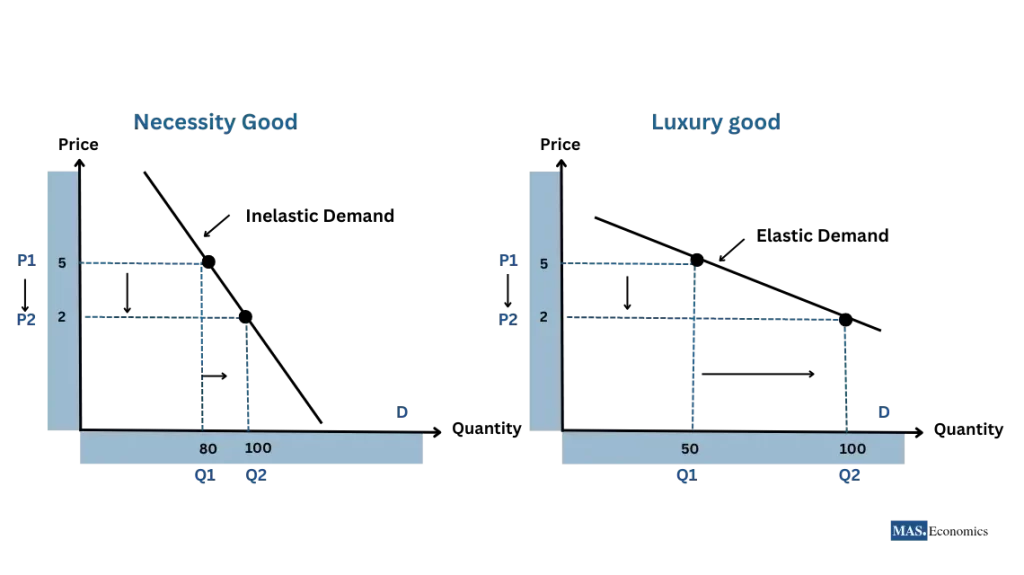
In the graph above, the steeper demand curve represents a necessity or other inelastic good – quantity doesn’t change much with price. The flatter demand curve represents a luxury or highly substitutable good – quantity is very sensitive to price changes. This illustrates that not all products respond to price changes in the same way.
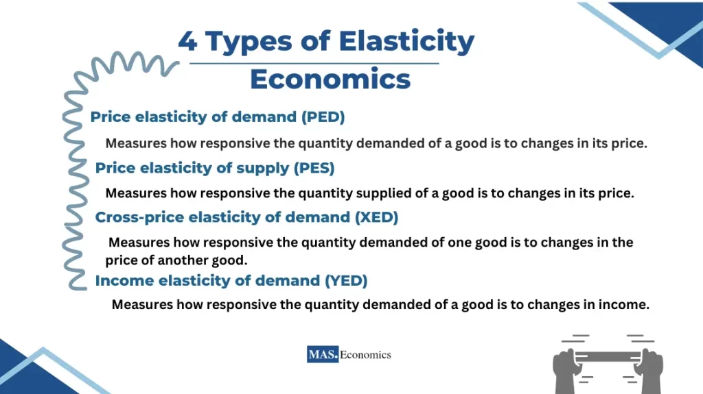
There are four main types of elasticity economists focus on:
Price Elasticity of Supply (PES) – how the quantity supplied responds to price changes.
Price Elasticity of Demand (PED) – how the quantity demanded responds to price changes of the same good.
Cross-Price Elasticity of Demand (XED) – how the quantity demanded of one good responds to price changes of another good (substitutes or complements).
Income Elasticity of Demand (YED) – how the quantity demanded changes as consumer income changes.
For a quick overview, refer to the table below summarizing the formulas, typical ranges, and real-world examples for each elasticity type.
Key Elasticity Measures Overview
| Elasticity Type | Formula | Interpretation / Typical Range | Real-World Example |
|---|---|---|---|
| Price Elasticity of Demand (PED) | \( PED = \frac{\% \Delta Q_d}{\% \Delta P} \) | Elastic: >1; Inelastic: <1; Unit Elastic: =1 (note: typically negative due to inverse relation) |
Luxury smartphones: PED ≈ −1.6 |
| Cross-Price Elasticity (XED) | \( XED = \frac{\% \Delta Q_d^A}{\% \Delta P^B} \) | >0: Substitutes; <0: Complements; ≈0: Unrelated goods | Smartphones & phone cases: XED ≈ −0.53 |
| Income Elasticity of Demand (YED) | \( YED = \frac{\% \Delta Q_d}{\% \Delta Income} \) | >1: Luxuries; 0–1: Necessities; <0: Inferior goods | Luxury cars: YED ≈ +2.0; Instant ramen: YED ≈ −0.5 |
| Price Elasticity of Supply (PES) | \( PES = \frac{\% \Delta Q_s}{\% \Delta P} \) | >1: Elastic; <1: Inelastic; =1: Unit Elastic | Smartphones: PES ≈ 2.5; Wheat: PES ≈ 0.25 |

|
|||
In the rest of this article, we’ll explore each of these elasticity types in detail, with formulas, examples, and their real-world implications.
Price Elasticity of Demand (PED)
Price Elasticity of Demand (PED) measures how responsive the quantity demanded of a good is to a change in its own price. Formally, it’s the percentage change in quantity demanded divided by the percentage change in price:
\( PED = \frac{\% \Delta \text{Quantity Demanded}}{\% \Delta \text{Price}} \)
This formula typically yields a negative value because of the inverse relationship between price and demand (when price goes up, quantity demanded goes down, and vice versa). Economists often interpret PED in absolute terms (ignoring the negative sign) when categorizing demand as elastic or inelastic.
Example calculation: Suppose a luxury smartphone brand drops the price of its flagship phone from $800 to $700 (a price decrease of $100). As a result, the quantity demanded rises from 1,000 units to 1,200 units. Let’s calculate the PED step by step:
- Initial price: $800
- New price: $700
- Initial quantity demanded: 1,000 units
- New quantity demanded: 1,200 units
The percentage change in price is \( \frac{700 – 800}{800} = -0.125 \), or -12.5% (negative because it’s a price decrease).
The percentage change in quantity demanded is \( \frac{1200 – 1000}{1000} = 0.20 \), or +20%.
Now plug these into the formula for PED:
\( PED = \frac{+20\%}{-12.5\%} \approx -1.6 \)
The PED comes out to approximately –1.6. The negative sign here simply confirms the inverse relationship (price down, demand up). The magnitude 1.6 tells us the demand is quite responsive: a 1% drop in price leads to about a 1.6% increase in quantity demanded. In other words, this luxury smartphone has an elastic demand – consumers are pretty sensitive to its price.
When evaluating PED, we often focus on the absolute value and categorize the elasticity:
- Elastic Demand: PED > 1 (in absolute value). A small price change leads to a larger proportional change in quantity demanded. For instance, if PED = 2, a 5% rise in price would cause roughly a 10% drop in quantity demanded.
- Inelastic Demand: PED < 1. A price change causes a smaller proportional change in quantity demanded. For example, if PED = 0.5, a 10% increase in price only reduces quantity demanded by about 5%.
- Unit Elastic Demand: PED = 1. The percentage change in price is exactly matched by an equal percentage change in quantity. For example, a 10% price increase causes a 10% decline in quantity demanded.
(If PED = 0, demand is perfectly inelastic – quantity demanded doesn’t change at all when price changes (think of a life-saving medication with no substitutes). If PED is extremely high (approaching infinity), demand is perfectly elastic – even the slightest price increase would drop quantity demanded to zero, which is rare in practice.)
Determinants of Price Elasticity of Demand
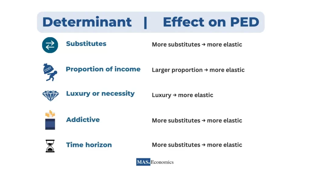
Several factors determine whether demand for a good is elastic or inelastic:
Availability of Substitutes
Goods with many close substitutes tend to have more elastic demand. If the price of one brand or option rises, consumers can easily switch to an alternative. For example, if the price of a popular soft drink goes up, many consumers will switch to another soda brand. On the other hand, if a good has few or no substitutes (like a unique medication or a monopolistic service), its demand will be more inelastic.
Necessities vs. Luxuries: Necessities
(like basic food, electricity, or insulin) usually have inelastic demand – people continue to buy them even when prices increase. For example, petrol (gasoline) has very few substitutes, so if its price rises sharply, the quantity demanded drops only slightly. In contrast, luxuries or non-essential goods (like high-end electronics, designer items, or sports cars) tend to have elastic demand – consumers can cut back or postpone these purchases if prices are too high. For instance, if the price of a luxury sports car (like a Porsche) increases, many potential buyers will delay buying or choose a different brand, making the demand much more sensitive to price.
Proportion of Income (Price Relative to Budget)
If a product consumes a large share of a consumer’s income, demand is likely to be more elastic. A significant price increase on an expensive item (say a car or a big-screen TV) makes a big dent in the budget, so people become more sensitive to price changes. Conversely, for inexpensive items that take a tiny fraction of income (salt, toothpaste), demand is usually inelastic because even doubling the price barely impacts someone’s finances.
Time Horizon
Demand often becomes more elastic over time. In the short run, consumers may not have time to find alternatives or change habits, so demand is less responsive to price changes. In the long run, they can adjust – finding substitutes or making lifestyle changes – making demand more responsive. For example, if gasoline prices spike suddenly, drivers might initially just pay more (short-run inelastic response). But over a year or two, they may carpool, use public transit, or switch to fuel-efficient cars, indicating a more elastic response in the long term.
Prices of Related Goods
The demand for a product can also be affected by changes in the prices of complementary goods. If a complement becomes more expensive, the product’s demand may fall. (This factor is essentially the realm of cross-price elasticity, which we discuss later.) For instance, if coffee prices skyrocket, the demand for coffee creamer may drop because fewer people are buying coffee.
(Note: The income level of consumers can also play a role. At higher income levels, people might be more flexible with luxuries and non-essentials, potentially making demand more elastic for those goods. Meanwhile, lower-income consumers might be more tightly constrained to necessities. However, this overlaps with the idea of necessity vs. luxury and how much of the budget a good consumes.)
These determinants work together to shape a product’s elasticity. For example, gasoline is a necessity with few substitutes (especially in the short term), so its demand is notoriously inelastic. Studies show that in the short run, even a 25–50% drop in gas prices would raise consumption only by about 1%. By contrast, air travel for vacations is a luxury purchase with alternatives, making its demand more elastic – a 10% fare increase can cut vacation air travel by more than 10%.
Applications of Price Elasticity of Demand
Understanding PED is extremely useful for different economic agents:
Governments
Policymakers use PED to design taxes and subsidies. If the government wants to raise revenue, it will often tax goods with inelastic demand (like tobacco or gasoline) because consumers will continue buying despite higher prices, resulting in stable tax revenue. However, if the goal is to discourage the consumption of something, taxing a good with elastic demand is more effective, as consumers will cut back a lot when the price rises. For example, a high tax on cigarettes (which have relatively inelastic demand) raises revenue, whereas a tax on luxury cars (more elastic demand) can sharply reduce their sales.
Businesses
Firms consider PED when setting prices and sales strategies. If demand for their product is elastic, a price reduction could sharply boost sales and potentially increase overall revenue (because the volume gained might outweigh the lower price per unit). But if demand is inelastic, a company might choose to increase the price to boost revenue, knowing that sales volume will drop only slightly. For instance, a software company might find that lowering the subscription price attracts many new customers (elastic demand), whereas an electricity utility knows it can charge a bit more without losing many customers (inelastic demand due to lack of substitutes).
Consumers
Savvy consumers can use elasticity knowledge for smart shopping. If a product has elastic demand, it’s likely to go on sale or have competitive pricing, so waiting for a discount or shopping around can pay off. But for products with inelastic demand (essential goods you need now), waiting for a sale might not be worthwhile since prices are less likely to drop and you need the item regardless. For example, if you know electronics tend to have sales, you might wait for Black Friday to buy a TV (elastic demand). But if you need a prescription medicine (inelastic demand), you’ll have to buy it even if the price is high.
Market Researchers and Economists
Elasticity helps analysts understand consumer behavior patterns. By studying PED, market researchers can gauge how consumers might react to price changes, which in turn helps in forecasting sales and crafting marketing strategies. It also aids economists in predicting the impact of market shocks. For example, researchers might use elasticity estimates to predict how a sudden increase in food prices will affect consumption and nutrition levels in a community.
Cross-Price Elasticity of Demand (XED)
While PED deals with a good’s response to its own price, Cross-Price Elasticity of Demand (XED) measures how the quantity demanded of one good changes when the price of another good changes. This is crucial for understanding substitute and complement relationships between products. The formula for cross-price elasticity is:
\( XED = \frac{\% \Delta \text{Quantity Demanded of Good A}}{\% \Delta \text{Price of Good B}} \)
- If XED is positive, the two goods are substitutes: an increase in the price of Good B increases demand for Good A (consumers switch from the now pricier B to A).
- If XED is negative, the goods are complements: an increase in the price of B decreases demand for A (the goods are used together, so pricier B means people buy less of A too).
- If XED is zero or near zero, the goods are mostly unrelated – a price change in one has no significant effect on demand for the other.
Example: Let’s say Good A is smartphone cases and Good B is smartphones. If smartphone prices rise by +15%, and as a result the quantity of phone cases demanded falls by –8% (because fewer people are buying new phones, so case purchases drop), then:
\( XED = \frac{-8\%}{+15\%} \approx -0.53 \)
The XED is –0.53, a negative number, indicating these goods are complements (which makes sense: phones and phone cases go together). The magnitude 0.53 is moderate; it means a 1% increase in phone prices leads to about a 0.53% decrease in case purchases.
Now consider substitute goods. Imagine coffee and tea are substitutes for many people. If the price of coffee goes up, some people will buy more tea instead. Suppose coffee becomes 10% more expensive, and tea demand rises by 5%. The XED for tea (Good A) with respect to coffee (Good B) would be +0.5, indicating a substitute relationship.
Determinants of Cross-Price Elasticity
What influences the cross-price elasticity between two goods?
Closeness of Substitutes
If two goods are very similar or fulfill the same need, they have a high positive XED. For example, butter and margarine are close substitutes – a jump in butter prices can cause a significant increase in margarine demand. On the other hand, butter and olive oil might be less substitutable in certain recipes, so their XED would be lower.
Strength of Complementarity
If goods are usually consumed together, they’ll have a high-magnitude negative XED. For instance, printers and ink cartridges are strong complements – if printers get cheaper, people buy more printers and thus more ink, and vice versa. In contrast, an increase in car prices might only slightly reduce demand for gasoline in the short run because many car owners still need gas (the complementarity is strong, but necessity can moderate the effect).
Time Horizon
As with PED, time matters. In the short run, consumers might not immediately change their behavior when the price of a related good changes (leading to a lower immediate XED). Over the long run, they have more time to adjust their consumption habits. For example, if gasoline prices remain high for years, more people may switch to electric vehicles, drastically reducing gasoline demand (a long-run complement effect). In the very short term, a rise in gas prices might not instantly reduce car usage much (low short-run complementarity effect).
Market Definition and Availability of Alternatives
If there are many alternative complements or substitutes, any given pair’s XED might be lower because consumers have multiple ways to adjust. For example, if the price of one brand of coffee increases, a coffee drinker might also consider switching to tea, energy drinks, or other sources of caffeine, diffusing the impact on any single substitute like tea.
Applications of Cross-Price Elasticity
Understanding XED helps businesses and policymakers make strategic decisions:
Pricing and Product Strategy
Companies with product lines of related goods must consider cross elasticity. A price change in one product could impact the sales of another. For instance, a company selling game consoles and video games (complements) might price the console low to boost game sales. Conversely, a firm that sells two substitute products may avoid pricing them such that one cannibalizes the other’s sales. If XED is high between your product and a rival’s product (strong substitutes), raising your price could send customers straight to the competitor. Businesses often research cross elasticity to anticipate such effects.
Marketing and Bundling
Knowledge of complements and substitutes can guide marketing campaigns. For complementary goods, businesses might bundle products or do co-promotions (e.g., offering a discount on phone cases with a phone purchase) to capitalize on the relationship. For substitutes, marketing needs to highlight differentiators. If a competing product becomes more expensive, it might be a good time to advertise your product as an attractive alternative.
Policy Making
Governments consider cross elasticity when evaluating the broader impact of taxes or subsidies. For example, if the government taxes gasoline heavily (to reduce usage or raise revenue), it should anticipate effects on related markets: demand for fuel-efficient cars, public transportation usage, or complementary products like motor oil might change too. Similarly, if e-cigarettes and traditional cigarettes are substitutes, regulations or taxes on one will affect consumption of the other, which is important for public health policy planning.
Income Elasticity of Demand (YED)
Income Elasticity of Demand (YED) measures how the quantity demanded of a good responds to changes in consumers’ income. The formula is:
\( YED = \frac{\% \Delta \text{Quantity Demanded}}{\% \Delta \text{Income}} \)
Depending on the sign and magnitude of YED, goods are categorized as normal goods or inferior goods, and further into necessities or luxuries:
Normal Good
YED is positive (> 0). When income rises, consumers buy more of the good. Most goods fall into this category, but the degree varies:
Necessity: YED is between 0 and 1. Quantity demanded rises with income, but at a lower percentage rate. For example, if your income goes up 10% and your spending on food rises only 4%, the YED for food is 0.4 – a necessity (you spend more when richer, but not massively more). Food is a classic necessity; as incomes rise, households’ demand for food increases less than proportionally (Engel’s Law).
Luxury: YED > 1. Quantity demanded rises more than proportionally with income. For instance, a 10% income increase might lead to a 20% increase in demand for overseas vacations (YED = 2.0). High-end goods like luxury cars, designer clothing, or fine dining tend to have YED > 1 – people splurge more on them as they become wealthier.
Inferior Good
YED is negative (< 0). Demand for the good falls when income rises. This happens with goods that people buy out of necessity when incomes are low, but abandon in favor of better alternatives as soon as they can afford to. For example, public transportation can be an inferior good – as people’s incomes grow, they might use buses or trains less and start driving cars instead. In one study, the income elasticity of demand for public transit was about –0.36, indicating that an increase in income led to a decrease in public transport usage.
Example: Imagine the average income in a city increases by +10% this year. A luxury car dealership observes that annual sales of their cars rise from 500 to 600 units (that’s a +20% increase in quantity sold). The YED for these luxury cars would be:
\( YED = \frac{+20\%}{+10\%} = +2.0 \)
A YED of +2.0 indicates a luxury normal good – demand grows twice as fast as income. This makes sense for luxury cars: as people have more disposable income, their purchases of luxury vehicles climb significantly (they might buy a second car or upgrade to a premium model). On the other hand, consider an inferior good: if incomes rose 10% and the quantity demanded of instant ramen noodles dropped by 5%, the YED for ramen would be –0.5, reflecting its inferior good status (people upgrade to better meals as soon as they can)
With its sign, YED helps illuminate the nature of goods in the context of income changes:
Necessities
These are life’s essentials; demand for them remains relatively stable as income fluctuates. Think of food and housing — vital for survival — where quantity demanded doesn’t change drastically with income. (You won’t eat double the meals because your salary doubled; you’ll just maybe buy slightly better or more varied food.)
Luxuries
The demand for luxuries dances with income variations, often growing more than proportionally as people earn more. Vacations and jewelry are good examples — not vital for survival, but as income grows, people indulge much more in these items.
Inferior Goods
These thrive only when prosperity is lacking. As income increases, demand for inferior goods drops, since consumers switch to preferred alternatives. Examples include cheap instant foods or second-hand products that people replace with higher-quality options once they can afford to.
Determinants of Income Elasticity of Demand
Key factors influencing YED include:
Type of Good (Necessity, Luxury, Inferior)
As discussed above, whether a good is essential, a luxury, or a lower-end substitute determines how demand shifts with income. Basic necessities have low positive YED, luxuries have high positive YED, and inferior goods have negative YED.
Consumer Preferences and Culture
In different contexts, the same good might have a different income elasticity. For example, in a developing economy, owning a car might be considered a luxury (high YED), whereas in a high-income country it might be seen as a necessity (lower YED). Cultural norms and preferences also influence what people do with extra income.
Price Level of the Good
The baseline price of the good can interact with income effects. If a good is extremely expensive (like real estate or luxury artwork), even wealthier consumers might not dramatically increase the quantity they buy as their income grows (you might buy a nicer house, but not many houses). This could moderate the YED for very high-ticket items. Conversely, for affordable treats or mid-range goods, higher income might translate into buying significantly more units or upgrading quality, reflecting a higher YED.
Income Distribution and Stage of Life
The same product can have different elasticity for different income groups or age groups. For a young professional whose income is rising, a pay raise might strongly increase spending on dining out or new gadgets. For a millionaire, the same percentage income increase might not change consumption at all (diminishing marginal propensity to consume). Similarly, younger consumers might allocate new income differently than older consumers. This touches on how life cycle stages affect YED (e.g., young adults might have a higher YED for housing than retirees, since housing consumption for an older person may already be at a comfortable maximum).
Applications of Income Elasticity
Business Strategy (Pricing & Production)
Businesses tailor their strategies according to the YED of their products. If a product has a high YED, its sales will be closely tied to economic booms and busts. Companies selling luxury or premium goods (high YED) might ramp up production and marketing in good economic times when incomes are rising, and prepare for leaner times during recessions. They might also adjust pricing during different economic conditions — for instance, offering more financing options or entry-level models in downturns. In contrast, producers of necessities (low YED) know that demand is steadier across economic cycles, so their production and inventory planning can be more stable.
Marketing Focus
Marketing can be directed to the right audience using YED insights. Luxury brands often target high-income segments and emphasize exclusivity when the economy is strong. If a brand knows a certain product is an inferior good, it will market it in value-focused channels and be prepared for demand to drop in more affluent segments. For normal goods, messaging can be adjusted with economic conditions: a mid-range car manufacturer might highlight affordable reliability during recessions, but during boom times, it might promote premium upgrades since consumers have more to spend.
Policy Making
Governments and public institutions pay attention to income elasticity for various goods to craft policies. For example, if the government knows that public transit is an inferior good (negative YED), then during economic downturns (when incomes fall), more people will rely on public transportation, so they might need to invest more in it. Conversely, luxury goods often become targets for luxury taxes since higher-income individuals can afford to pay and such taxes don’t significantly affect lower-income households. Additionally, understanding which goods are necessities with low YED (like basic food staples) can guide subsidy and welfare policies — ensuring those items remain accessible as incomes vary.
Application in Practice
Consider a business specializing in gourmet organic foods. These items are likely luxury goods with a high YED — when consumers have higher incomes, they significantly increase spending on organic and premium foods. Recognizing this, the business might expand its product line or raise prices slightly during economic boom periods when customers are more willing to pay for premium quality. However, the company must be cautious during economic downturns: a slight drop in average incomes could sharply reduce demand for expensive organic products as consumers switch back to cheaper alternatives.
Price Elasticity of Supply (PES)
We’ve examined how demand reacts to various changes; now let’s turn to Price Elasticity of Supply (PES), which measures how responsive the quantity supplied of a good is to a change in its price. The calculation is analogous to PED, but from the supplier’s perspective:
\( PES = \frac{\% \Delta \text{Quantity Supplied}}{\% \Delta \text{Price}} \)
PES is usually positive because price and quantity supplied move in the same direction (a higher price generally encourages producers to supply more). The value indicates how easily producers can change production in response to price shifts:
- Elastic Supply: PES > 1. Producers can ramp production up or down quickly. A small price increase leads to a larger percentage increase in quantity supplied.
- Inelastic Supply: PES < 1. Producers find it hard to change production in the short term. Even a large price rise might result in only a small increase in quantity supplied.
- Unit Elastic Supply: PES = 1. A percentage change in price leads to an equal percentage change in quantity supplied.
To illustrate elastic vs inelastic supply, consider the following scenarios along with the supply curves shown in the graph below:
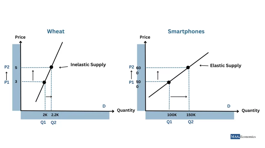
In the graph, the steeper supply curve might represent a crop like wheat in the short run. Farmers can’t quickly increase the harvest just because prices jumped – they’re limited by the planting season and land available. The flatter supply curve might represent an assembled product like smartphones, where factories can relatively quickly add an extra shift or increase output when prices (and profitability) rise.
Example 1 (Inelastic Supply – Agriculture): Suppose a poor harvest causes wheat prices to rise from $5 to $7 per bushel. Farmers worldwide scramble to supply more because of the higher price, and the total quantity supplied in the market goes up from 2,000 bushels to 2,200 bushels. That’s a +40% price increase, but only a +10% increase in quantity. Using the PES formula:
\( PES_{\text{wheat}} = \frac{+10\%}{+40\%} = 0.25 \)
A PES of 0.25 is quite inelastic. It means a 1% increase in price yields only a 0.25% increase in quantity supplied. In practical terms, wheat farmers can’t quickly boost output in response to a price spike. They’re constrained by factors like growing time and available farmland. If prices remain high, over a longer period farmers may plant more next season or new suppliers may enter the market, but in the short run, supply is sluggish to respond.
Example 2 (Elastic Supply – Manufactured Good): Now consider smartphones. Suppose a surge in consumer demand drives the market price of smartphones up from $500 to $600 on average (a +20% increase), and manufacturers respond by increasing production from 100,000 units to 150,000 units (a +50% increase in quantity). The PES would be:
\( PES_{\text{phones}} = \frac{+50\%}{+20\%} = 2.5 \)
A PES of 2.5 indicates elastic supply. Producers were able to greatly increase output when price rose. This is plausible because smartphone manufacturers might have some idle capacity or can add overtime shifts, so they can ramp up production relatively quickly as prices increase. As a result, the quantity supplied expands significantly with the price increase.
In summary, the wheat example shows inelastic supply – even a big price rise yields only a modest increase in quantity. The smartphone example shows elastic supply – a moderate price increase leads to a large jump in output.
Determinants of Price Elasticity of Supply
Several factors influence whether supply is elastic or inelastic:
Production Flexibility and Spare Capacity
If producers can change production levels easily, supply is more elastic. This could mean having extra factory capacity, flexible manufacturing processes, or inventory that can be tapped. For example, a factory running only one shift can add a second shift to double output if the price is right – indicating elastic supply. If all resources are already fully utilized, supply in the short term is inelastic until new capacity is added.
Time Horizon
Time is critical for supply adjustments. In the short run, at least one factor of production (e.g., factory space or number of fields) is fixed, so supply is often inelastic. Firms cannot instantly build a new factory or farmers cannot instantly grow more crops. In the long run, firms can expand capacity, new competitors can enter, and producers can adjust fully to price changes, making supply more elastic. For instance, if demand for electric cars suddenly surges, factories might not keep up this year (short-run inelastic supply), but given a few years, manufacturers will build new production lines and battery suppliers will increase capacity, resulting in much larger output (long-run elastic supply).
Availability of Inputs
If the inputs (raw materials, labor, components) needed to increase production are readily available, supply can be more responsive. If inputs are scarce or specialized, it’s harder to boost production, resulting in inelastic supply. For example, if a certain rare metal is required to make solar panels and that metal is in short supply, even if panel prices go up, producers can’t make many more panels without that key input. Conversely, if inputs and skilled labor are abundant, producers can increase output more easily when prices rise.
Degree of Specialization
If production facilities or skills are highly specialized for one product, supply might be less elastic because you can’t repurpose resources quickly. A factory that only produces one type of microchip can’t instantly switch to producing another product if its price becomes more attractive. Firms with flexible, multi-purpose technology or more generalized skills can adapt output as prices change, contributing to elasticity. Highly specialized industries often have high fixed costs and lead times, which make short-run supply inelastic.
Inventory and Storability
For goods that can be stored easily (non-perishables, commodities with long shelf-life), producers can respond to price changes by drawing from or adding to inventory. This makes supply more elastic in the short term because stockpiles can be sold when prices rise or held back when prices are low, smoothing out the response. Perishable goods or services (which cannot be stored) have to be produced when needed, often limiting short-run elasticity.
Applications of Price Elasticity of Supply
Pricing Strategy
Businesses consider PES when adjusting prices for their goods or services. If supply is very elastic in an industry, a small price cut might lead to a flood of additional output (as competitors or other suppliers ramp up production quickly), which could drive prices down further and hurt profits. On the flip side, if supply is inelastic, a company knows that increasing its price is less likely to be met by a surge of output from competitors in the short term, potentially making a price hike more profitable. In essence, firms in industries with highly elastic supply must be cautious with pricing, since the market can quickly be flooded. In industries with inelastic supply (at least in the short run), companies may have more pricing power.
Production and Capacity Planning
Firms use PES knowledge to plan production and capacity. If they operate in a market with elastic supply, they might keep production lean and wait for clear price signals, knowing they (and others) can scale up quickly if needed. If supply is inelastic, firms might invest in capacity in anticipation of higher prices, understanding that others can’t respond as fast – giving them an advantage when demand rises. For example, an oil company (where bringing new oil wells online takes time) might start new exploration projects if they anticipate higher oil prices, since short-run supply is inelastic. In contrast, a bakery (with relatively elastic supply of bread) will simply bake more if the price of bread rises, without needing long-term investments.
Government Policies
Governments examine PES to inform decisions on things like agriculture subsidies, resource extraction regulations, or import tariffs. If supply is very inelastic, a subsidy might not actually increase output much; it could just increase producers’ incomes. But if supply is elastic, a subsidy could significantly boost output and lower prices for consumers. For instance, if small farmers can quickly plant more crops given the right incentives, a subsidy or guaranteed price might lead to a large increase in food production (helping lower food prices). If farmers are already at capacity, the same policy might have little effect on quantity. Similarly, understanding PES helps in planning strategic reserves or responding to supply shocks – if an essential good has inelastic supply, the government might maintain a stockpile or encourage capacity expansion to avoid shortages.
Practical example: Imagine a small business selling handmade crafts. If the supply of these crafts is elastic (the owner can hire more artisans or use faster production methods), the business might confidently lower prices during a holiday sale, knowing they can produce enough to meet the surge in demand. However, if each item is one-of-a-kind art that takes a long time to make (inelastic supply), the business realizes that even if they raise prices, they cannot significantly increase output in the short run. Thus, they might keep prices higher and produce at a steady pace, focusing on quality over quantity.
Conclusion
Understanding elasticity is fundamental to grasping market dynamics. By measuring how quantity demanded or supplied responds to changes in price, income, or the prices of related goods, elasticity provides critical insights for economists, policymakers, and consumers alike. Whether a product is highly sensitive to price changes or remains largely unaffected, these measures help explain everyday economic behavior and guide strategic decisions. This article has explored the four key types of elasticity—price, cross-price, income, and supply elasticity—detailing their formulas, determinants, and real-world applications. A deep appreciation of these concepts not only clarifies how markets work but also empowers you to make informed pricing, production, and policy decisions in a constantly evolving economic landscape.
FAQs:
What is price elasticity of demand?
Price elasticity of demand (PED) measures how sensitive the quantity demanded of a product is to a change in its own price. It is calculated as the percentage change in quantity demanded divided by the percentage change in price. A higher absolute value indicates that demand is more responsive to price changes.
How is price elasticity of demand calculated?
It is computed using the formula \( PED = \frac{\% \Delta Q_d}{\% \Delta P} \). For example, if a product’s price falls by 12.5% and the quantity demanded increases by 20%, the PED would be approximately –1.6. The negative sign reflects the inverse relationship between price and quantity demanded, though we typically discuss the absolute value when describing elasticity.
What factors influence the elasticity of demand?
Several factors determine a product’s demand elasticity, including the availability of substitutes, whether the good is a necessity or a luxury, the proportion of a consumer’s income spent on the product, the time allowed for adjustment, and the effect of related goods’ prices. These factors collectively shape how consumers respond to price changes.
What does a negative value for PED signify?
A negative value for PED simply indicates the typical inverse relationship between price and demand—when price increases, quantity demanded decreases, and vice versa. While the negative sign is essential for the calculation, the absolute value is used to determine whether the demand is elastic or inelastic.
What is cross-price elasticity of demand (XED)?
Cross-price elasticity (XED) measures the responsiveness of the quantity demanded for one good when the price of another good changes. A positive XED suggests that the goods are substitutes, meaning an increase in the price of one leads to higher demand for the other. Conversely, a negative XED indicates that the goods are complements, so a price rise in one results in lower demand for the other.
How does income elasticity of demand (YED) differentiate between necessities and luxuries?
Income elasticity of demand (YED) measures how quantity demanded changes in response to changes in consumer income. For necessities, YED typically falls between 0 and 1, meaning that demand increases by a smaller percentage than income. For luxuries, YED is greater than 1, indicating that demand grows more than proportionally as income rises. If YED is negative, the product is considered an inferior good, meaning demand falls as income increases.
What is price elasticity of supply (PES)?
Price elasticity of supply (PES) assesses how much the quantity supplied of a product changes in response to a change in its price. It is calculated as the percentage change in quantity supplied divided by the percentage change in price. A high PES shows that producers can adjust their output quickly when prices change, while a low PES indicates production is less responsive.
Why is understanding elasticity important for businesses and policymakers?
Elasticity is crucial because it provides insights into market behavior—helping businesses set optimal pricing and production levels, and guiding policymakers in designing effective taxes, subsidies, and regulatory policies. Understanding elasticity helps predict how changes in prices or income will affect demand and supply, ultimately influencing revenue, consumer welfare, and market efficiency.
How do short-run and long-run elasticities differ?
In the short run, both demand and supply tend to be more inelastic because consumers and producers have limited time to adjust to price changes. Over the long run, as adjustments become feasible (such as finding substitutes or expanding production capacity), both demand and supply generally become more elastic.
Thanks for reading! If you enjoyed this series, spread the knowledge by sharing it with friends and on social media.
Happy learning with MASEconomics!