How to Select the Best Econometric Model for Your Data

In 1974, Hirotugu Akaike published a criterion that transformed model selection from an informal art into a likelihood‑based decision. Empirical economics demands choosing between competing specifications that explain the same phenomenon. Adding more regressors always improves the in‑sample fit, but it also captures random noise rather than true economic relationships. The best econometric model balances goodness of fit with parsimony, ensuring the estimates remain reliable for out‑of‑sample forecasting and policy analysis. Information criteria provide the mathematical framework for this balance. Without formal selection rules, empirical work drifts toward overfitting, mistaking sample‑specific idiosyncrasies for general economic laws.

Relying solely on R‑squared leads to overfitting. A model with too many parameters absorbs idiosyncratic variations in the sample data, causing the estimates to change drastically when applied to new observations. Model selection criteria like the Akaike Information Criterion and the Bayesian Information Criterion solve this by imposing a penalty for complexity. They evaluate whether the marginal improvement in fit justifies the addition of another parameter, transforming a subjective comparison of fit statistics into a rigorous probabilistic decision.

Why Adding Variables Fails

In multiple regression models, adding an independent variable never reduces the R-squared. This mathematical property creates a false incentive to include as many regressors as possible. However, every additional parameter consumes a degree of freedom and increases the variance of the remaining estimators. When the sample size is limited, including irrelevant variables makes the coefficient estimates less precise, widening the confidence intervals and obscuring the true economic relationships.

The bias-variance tradeoff explains the core problem. A simple model underfits the data, producing biased estimates because it omits relevant variables. A complex model overfits the data, producing high-variance estimates that fluctuate wildly with small changes in the sample. The optimal model exists at the point where the reduction in bias from adding a variable equals the increase in variance. Information criteria operationalize this tradeoff by penalizing the loss of degrees of freedom.

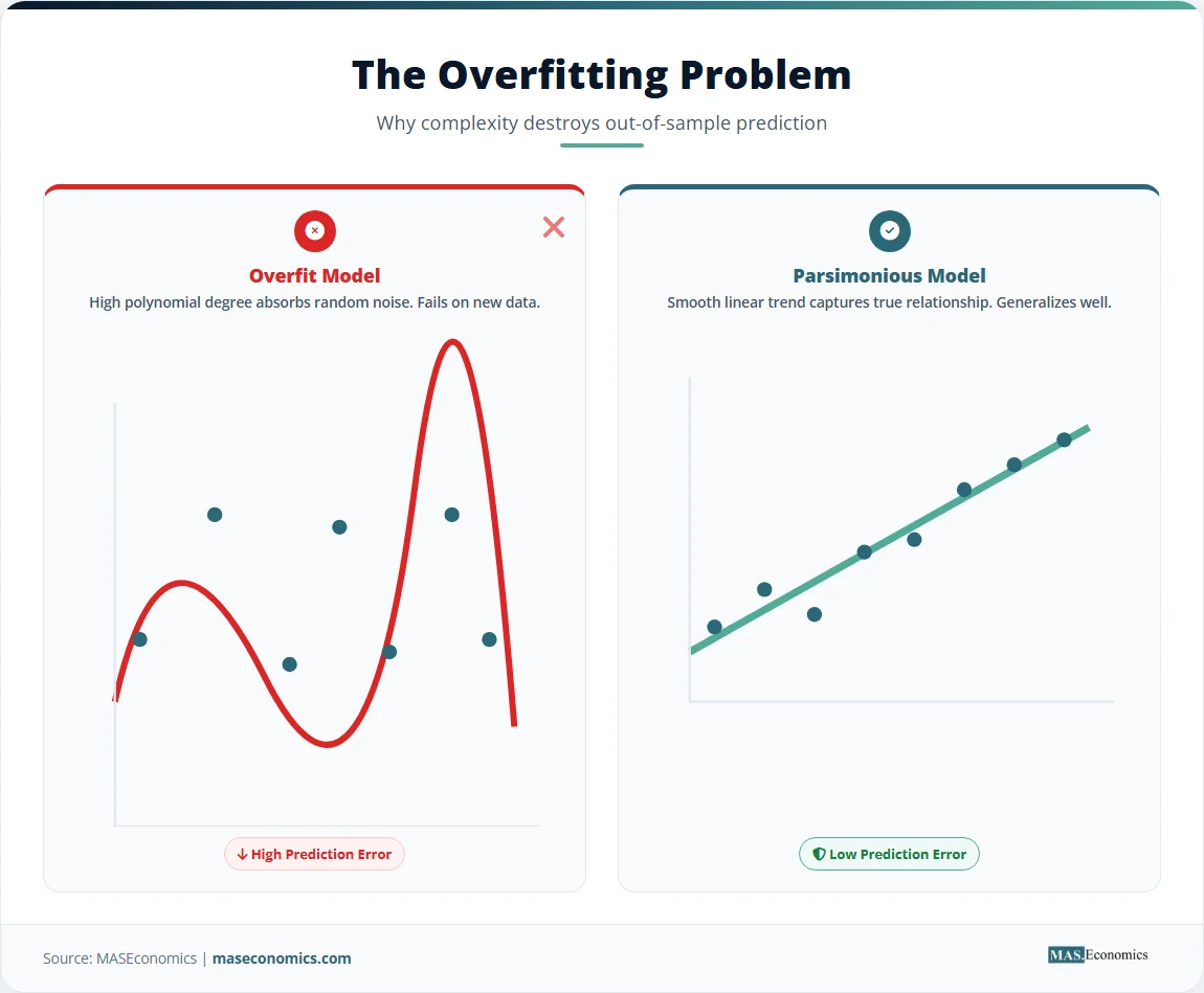
Overfitting occurs when a model captures the random fluctuations of the sample rather than the underlying data generation process. An overfit model yields impressive in-sample statistics but fails completely when applied to out-of-sample data. The simple linear regression framework illustrates this clearly. A scatter plot might show a slight wobble that a polynomial curve could fit perfectly, but the straight line almost always forecasts the next observation better because the wobble was just noise.

Adjusted R-squared attempts to fix the problem by penalizing the addition of irrelevant variables. It only increases when a new regressor improves the fit more than would be expected by chance. The formula divides the sum of squared residuals by the degrees of freedom:

While adjusted R-squared penalizes complexity, it relies on a specific penalty formula that does not map cleanly to probability theory. Information criteria ground the penalty in the log-likelihood function, providing a rigorous probabilistic foundation for model comparison. The foundations of econometrics rely on these likelihood-based methods to ensure statistical validity.

AIC and BIC: Penalty‑Based Selection

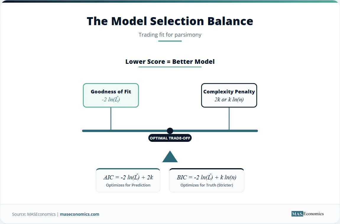
The Akaike Information Criterion (AIC) and the Bayesian Information Criterion (BIC) transform the model selection problem into an optimization task. Both criteria evaluate the maximized log-likelihood of the model and subtract a penalty term that increases with the number of parameters. A lower value indicates a better model.

The AIC estimates the relative distance between the true data generation process and the fitted model. Let \( \hat{L} \) denote the maximized value of the likelihood function, \( k \) the number of estimated parameters, and \( n \) the sample size. The AIC formula is:

The first term, \( -2 \ln(\hat{L}) \), measures the lack of fit. A model that fits the data perfectly yields a high likelihood, making this term small. The second term, \( 2k \), is the complexity penalty. Every additional parameter adds a penalty of 2. AIC selects the model that minimizes the combined score, effectively asking whether the improvement in fit outweighs the cost of estimating another parameter.

For linear regression models with normally distributed errors, the maximized log-likelihood relates directly to the sum of squared residuals (RSS). The AIC formula can be rewritten as:

The BIC approaches the problem from a Bayesian perspective. It estimates the posterior probability that a given model is the true model. The BIC formula is:

The BIC replaces the constant penalty of 2 with \( \ln(n) \). Because the natural logarithm of any sample size greater than 7 exceeds 2, BIC imposes a stricter penalty for complexity than AIC in most practical applications. As the sample size grows, BIC strongly favors parsimonious models. This strictness makes BIC a consistent model selection criterion, meaning that as the sample size approaches infinity, the probability of BIC selecting the true model approaches one. AIC does not share this property; it tends to select models that are slightly overparameterized, even with infinite data, trading consistency for predictive efficiency.

Consider a canonical example using cross-sectional wage data with 150 observations. Model 1 regresses log wages on education only. Model 2 regresses log wages on education and experience. The estimation yields the following fit statistics.

Table 1. Model Comparison: Wages on Education and Experience

Statistic	Model 1 (Education)	Model 2 (Education, Experience)
Parameters (k)	2	3
Sum of Squared Residuals	425.50	418.20
\( n \ln(RSS/n) \)	156.45	153.75
AIC	160.45	159.75
BIC	166.47	168.78

Note: Stylized canonical example. n=150.

Model 2 reduces the sum of squared residuals, yielding a better fit term of 153.75 compared to 156.45. AIC adds a penalty of 2 per parameter, meaning Model 2 receives a penalty of 6 versus a penalty of 4 for Model 1. The AIC for Model 2 is 159.75, which is lower than the AIC of 160.45 for Model 1. AIC selects the larger model because the fit improvement outweighs the slight penalty increase.

BIC applies a penalty of \( \ln(150) \approx 5.01 \) per parameter. Model 1 receives a BIC penalty of 10.02, while Model 2 receives a penalty of 15.03. The BIC for Model 2 is 168.78, which exceeds the BIC of 166.47 for Model 1. BIC selects the smaller model because the fit improvement does not justify the heavy complexity penalty. This divergence illustrates the fundamental difference between the two criteria.

Table 2 outlines the general decision rules for applying these criteria. When the criteria disagree, the choice depends on whether the analysis prioritizes forecasting accuracy or identifying the true data generation process.

Table 2. Model Selection: Decision Rules for AIC and BIC

Statistic Range	Decision
AIC(Model A) < AIC(Model B)	Select Model A for superior predictive accuracy
BIC(Model A) < BIC(Model B)	Select Model A for consistent true process identification
AIC favors complex, BIC favors parsimonious	Evaluate using out-of-sample validation and economic theory

Macro Forecasts and Policy Models

Central banks and international institutions rely heavily on information criteria to build macroeconomic models. The IMF World Economic Outlook forecasts depend on vector autoregressions that require precise lag length selection. Analysts use AIC and BIC to determine how many past quarters of data relevant macroeconomic variables contribute to current dynamics. Choosing too many lags consumes degrees of freedom and introduces noise, while too few lags omit important dynamics and cause autocorrelation in the residuals. The criteria provide an objective stopping rule for lag inclusion, preventing analysts from artificially boosting R-squared with irrelevant lagged variables.

The Federal Reserve faces similar challenges when modeling the Phillips curve to set monetary policy. Economists must decide whether to include expectations terms, supply shock variables, or structural break dummies. A National Bureau of Economic Research study demonstrates how information criteria help isolate the relevant inflation determinants without overfitting the historical data. The criteria prevent analysts from chasing spurious correlations that would lead to poor policy decisions. When evaluating competing macroeconomic theories, information criteria quantify the tradeoff between adding theoretical mechanisms and losing estimation precision.

The Bank for International Settlements applies model selection criteria when assessing the determinants of sovereign debt yields across countries. Because datasets span varying maturities, credit ratings, and liquidity measures, the risk of overfitting remains high. BIC helps identify a robust subset of variables that explain cross-country yield differentials without capturing country-specific noise. Similarly, the OECD Economics Department uses these criteria to select growth models that generalize across developed and developing nations, avoiding models that only fit the idiosyncrasies of a few large economies.

Labor economists also depend on model selection when estimating wage equations. A researcher might estimate a base model with education and experience, then test whether adding occupation dummies, regional indicators, or industry controls improves the specification. Information criteria determine whether the additional controls absorb meaningful variation or merely overfit the sample. When structural issues arise, such as heteroscedasticity or multicollinearity, the criteria must be applied to corrected specifications to ensure the fit measures remain valid. Failure to correct for heteroscedasticity before calculating information criteria renders the comparison meaningless because the likelihood function is misspecified.

Where Information Criteria Mislead

Information criteria provide a rigorous mathematical comparison, but they possess strict limitations. The criteria only evaluate the relative quality of the models presented to them. If all the candidate models are fundamentally misspecified, AIC and BIC will merely select the least bad option. The selected model might still fail standard diagnostic tests for normality, serial correlation, or structural breaks. Analysts must verify that the chosen specification passes relevant mis-specification tests before interpreting the information criterion result as a validation.

BIC assumes that the true model lies within the set of candidate models. In economics, this assumption rarely holds. Economic systems are complex, and all econometric models are simplifications. When the true model is not in the candidate set, BIC can be overly restrictive, shedding variables that improve predictive accuracy. AIC does not assume the true model is in the set, which makes it more robust for prediction but prone to including irrelevant variables in the pursuit of marginal fit improvements. This difference explains why forecasting applications often prefer AIC, while structural identification exercises prefer BIC.

In small samples, both criteria can behave unpredictably. The penalty terms in AIC and BIC are derived from asymptotic approximations. When the number of observations is limited relative to the number of parameters, these approximations break down. A small-sample correction for AIC, known as AICc, adds an extra penalty term that intensifies as the sample size shrinks relative to the parameter count.

When the sample size is small, the second term grows large, heavily penalizing complex models. As the sample size increases, the correction term approaches zero, and AICc converges to AIC. Analysts should prefer AICc in any situation where the number of parameters constitutes a substantial fraction of the sample size.

Information criteria also struggle with non-nested models. When Model A is not a special case of Model B, standard likelihood ratio tests cannot compare them. AIC and BIC allow non-nested comparisons, but the interpretation changes. The criteria measure the distance from the true process to each candidate, but they cannot assign a probability to the hypothesis that Model A is true versus Model B. Bayesian model averaging provides a more complete framework for non-nested comparison by weighting estimates across all candidate models according to their posterior probabilities.

Finally, model selection criteria cannot replace economic theory. A model might achieve a lower AIC than its competitors while implying a negative effect of education on wages. Such a result violates decades of labor economics research. Statistical criteria identify patterns in the data, but they cannot distinguish causal relationships from confounding factors. Instrumental variables and natural experiments remain necessary to establish causality. An algorithm cannot substitute for institutional knowledge.

MASEconomics Explains

Conclusion

The best econometric model balances goodness of fit with parsimony by penalizing unnecessary complexity. The Akaike Information Criterion optimizes for out-of-sample prediction, while the Bayesian Information Criterion optimizes for identifying the true data generation process. Both criteria transform model selection from a subjective comparison of R-squared values into a rigorous, likelihood-based decision. However, information criteria cannot substitute for economic theory or diagnostic testing. A lower score does not guarantee that the model satisfies the Gauss-Markov assumptions or implies a causal relationship. Combining statistical criteria with theoretical logic remains the soundest approach to empirical modeling.

Thank you for reading! If you found this helpful, share it with friends and spread the knowledge. Happy learning with MASEconomics