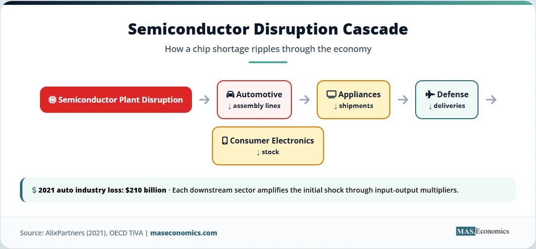
When a fire at a single Taiwanese semiconductor plant disrupts production for a few weeks, the damage does not stay in the tech sector. Automakers idle assembly lines because dashboard chips are missing. Appliance manufacturers delay washing machine shipments. Defense contractors miss delivery deadlines on radar systems. A 2021 chip shortage triggered by exactly this kind of disruption cost the global auto industry an estimated $210 billion in lost revenue, according to AlixPartners.
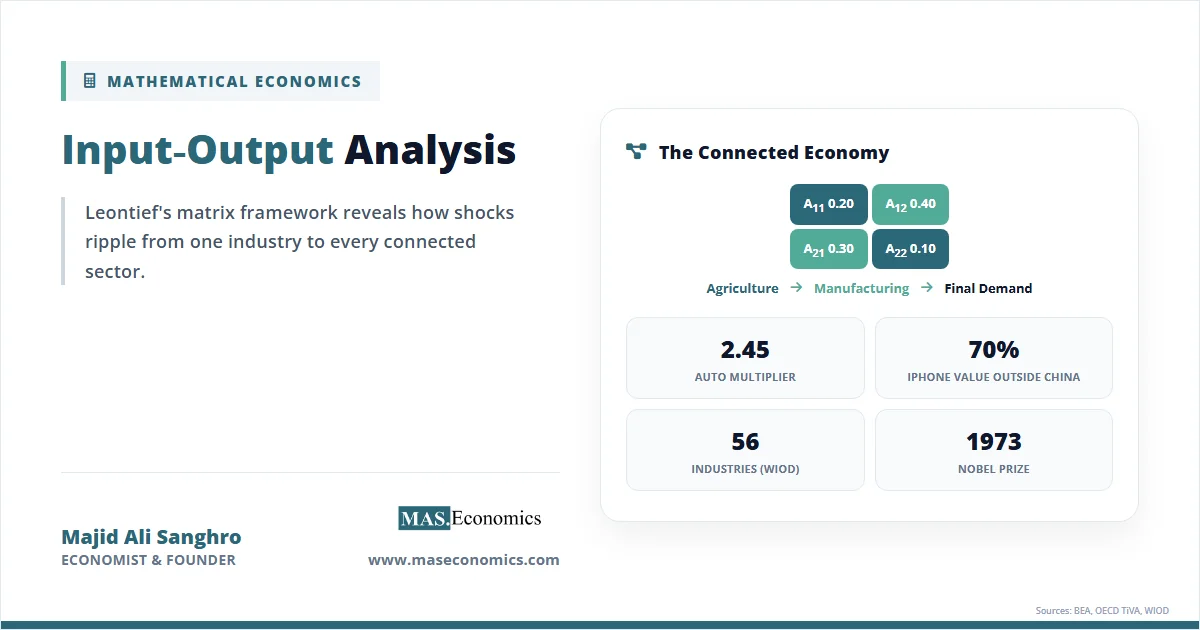
Input-output analysis economics is the formal framework that traces these domino effects. Built by Wassily Leontief in the 1930s and recognised with the 1973 Nobel Prize, it maps how every industry’s output becomes another industry’s input, and quantifies how a shock in one corner of the economy ripples through every connected sector.
The framework converts a tangle of supply relationships into a single matrix. Once that matrix is in hand, an economist can answer questions that look impossible from the outside: how much steel is embedded in a car, how many jobs depend on the construction sector, how a tariff on imported chemicals raises costs for pharmaceuticals and textiles at the same time.
Input-Output Analysis Defined
Input-output analysis is a quantitative method that represents an economy as a system of linked industries, where the output of each industry is partly consumed by households and government and partly used as an input to other industries. Wassily Leontief introduced the technique in his 1936 paper “Quantitative Input and Output Relations in the Economic System of the United States,” published in the Review of Economics and Statistics.
The core data object is the input-output table. Rows record how industry i sells its output: some goes to industry 1, some to industry 2, some to final demand (households, exports, government). Columns record what industry j buys: raw materials from agriculture, energy from utilities, services from finance, plus value added (wages and profits). The table balances by construction, since every dollar of output is also a dollar of someone’s expenditure, mirroring the logic explored in measuring national income.
Two derived objects do most of the analytical work. The first is the technical coefficients matrix \( A \), where each entry \( a_{ij} \) measures the dollars of input from industry i needed to produce one dollar of output in industry j. The second is the Leontief inverse, \( (I-A)^{-1} \), which captures both direct and indirect requirements. When final demand for cars rises by one unit, the Leontief inverse tells you not only how much steel is needed for those cars, but also how much coal is needed for that steel, how much electricity is needed for that coal, and so on through every round of production.
The Mechanics of the Model
Start with the accounting identity. Total output \( x_i \) of industry i equals sales to other industries plus sales to final demand:
where \( z_{ij} \) is the dollar value of industry i’s output used by industry j, and \( f_i \) is final demand for industry i’s output. Leontief’s key step was to assume that intermediate use scales linearly with output. Define the technical coefficient:
This is the input requirement per dollar of output in industry j. With \( z_{ij} = a_{ij} x_j \), the identity becomes:
In matrix form, with \( x \) and \( f \) as column vectors and \( A \) as the \( n \times n \) coefficient matrix:
Solving for \( x \):
The matrix \( L = (I-A)^{-1} \) is the Leontief inverse. Each entry \( l_{ij} \) gives the total output of industry i required, directly and indirectly, to deliver one dollar of final demand for industry j’s product. Column sums of \( L \) are backward linkages; row sums are forward linkages.
A Two-Sector Worked Example
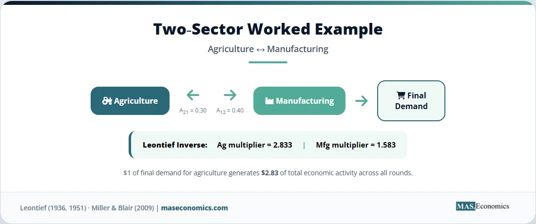
Take a small economy with two industries: agriculture and manufacturing. Suppose producing $1 of agricultural output requires $0.20 of agricultural inputs (seed, feed) and $0.30 of manufactured inputs (fertiliser, tractors). Producing $1 of manufactured output requires $0.40 of agricultural inputs and $0.10 of manufactured inputs. Final demand is $100 for agriculture and $200 for manufacturing.
The technical coefficients matrix is:
Then \( I-A = \begin{pmatrix} 0.80 & -0.40 \\ -0.30 & 0.90 \end{pmatrix} \), with determinant \( 0.80 \times 0.90-(-0.40)(-0.30) = 0.72-0.12 = 0.60 \).
The Leontief inverse is:
Total output is then:
Agriculture needs to produce $283.30 to deliver $100 of final demand, because the rest is absorbed as intermediate input by both sectors. Manufacturing needs to produce $316.70 to deliver $200 of final demand. The multipliers are 2.833 and 1.583, respectively, meaning each dollar of final agricultural demand triggers $2.83 of total economic activity once indirect rounds are counted.
| Symbol | Meaning | Example Value |
|---|---|---|
| \( x_i \) | Total output of industry i | Agriculture: 283.3; Manufacturing: 316.7 |
| \( f_i \) | Final demand for industry i | Agriculture: 100; Manufacturing: 200 |
| \( z_{ij} \) | Sales from industry i to industry j | \( z_{12} = a_{12} x_2 = 126.7 \) |
| \( a_{ij} \) | Input from i needed per $1 of output in j | \( a_{12} = 0.40 \) |
| \( A \) | Technical coefficients matrix | 2 × 2 matrix above |
| \( I \) | Identity matrix | 2 × 2 identity |
| \( (I-A)^{-1} \) | Leontief inverse: total requirements | Multiplier matrix above |
| Backward linkage | Column sum of Leontief inverse | Agriculture: 2.00; Manufacturing: 2.00 |
| Forward linkage | Row sum of Leontief inverse | Agriculture: 2.167; Manufacturing: 1.833 |
 | ||
Table 1. Variables and Values: Two-Sector Leontief Example.
Where the Numbers Come From
Real input-output tables are built from production censuses, supply-use tables, and tax records, then balanced and reconciled. The US Bureau of Economic Analysis input-output accounts publish detailed tables with 71 summary industries and 405 detailed industries, updated annually with a five-year benchmark revision drawn from the Economic Census. The construction work is enormous, but the resulting matrix lets analysts run thousands of counterfactuals from a single dataset.
Assumptions of the Leontief Model
The Leontief framework rests on three strong assumptions, and each one points to where the model breaks.
The first is fixed input coefficients. If steel becomes expensive, the model says automakers still use the same amount of steel per car. There is no substitution for aluminium or composites. This works tolerably well for short-run analysis where capital is fixed, but it overstates rigidity for longer horizons. A 2018 IMF working paper on production networks documents how substitution elasticities matter once input prices move significantly.
The second is constant returns to scale. Doubling output requires doubling every input in the same proportion. Real production functions, including the Cobb-Douglas form, often allow increasing or decreasing returns. For most short-run questions, this matters less than the substitution issue, but it constrains how the model handles big structural changes.
The third is the static frame. The basic model takes a snapshot of the economy and asks what would happen if final demand changed today, given today’s technology. It does not endogenise capital accumulation, technical change, or price adjustment.
Three families of extensions address these limits. Dynamic input-output models, developed by Leontief himself in the 1950s, add capital coefficients so that investment in one period feeds productive capacity in the next. Multi-regional input-output (MRIO) models split each industry by country or region, capturing global supply chains in a single matrix. Environmental input-output analysis appends rows for emissions, water use, or land use, allowing carbon footprints to be traced through the supply chain. Computable general equilibrium (CGE) models go furthest, replacing fixed coefficients with explicit production and utility functions and allowing prices to clear markets.
The Data Behind the Model
Three datasets dominate modern input-output empirical work. The World Input-Output Database (WIOD) covers 43 countries and 56 industries with consistent time series from 2000 to 2014, and an extended release through 2018. The OECD Trade in Value Added (TiVA) database covers 76 economies and 45 industries, with a focus on decomposing gross trade into domestic and foreign value added. The Eurostat supply, use, and input-output tables provide harmonised data for European economies.
The most striking empirical finding from this data is the chasm between gross and value-added trade. The classic example is the iPhone. A 2010 study by Kraemer, Linden, and Dedrick, later updated by the OECD Global Value Chains analysis, found that although iPhones were assembled in China and counted as Chinese exports in conventional trade statistics, only a small share of the device’s value was actually added in China. The bulk came from components produced in Japan, South Korea, the United States, Germany, and Taiwan. China’s role was final assembly, capturing roughly 5 to 10 percent of the retail value, while the bilateral US-China trade deficit was credited with the full $400-plus retail price per phone.
The TiVA framework formalised this insight across all goods. When the OECD recomputed trade balances in value-added terms, the US-China bilateral deficit shrank by about a quarter, because Chinese exports to America embodied significant Korean, Japanese, and German content. The bilateral deficit narrative looked very different once intermediate inputs were properly attributed.
Recent applications include carbon accounting. The EXIOBASE multi-regional environmental input-output database attributes CO\(_2\) emissions to the country of final consumption rather than the country of production. Studies using this approach show that high-income countries are larger net importers of embodied emissions than their domestic production statistics suggest, complicating any simple narrative about who is responsible for global emissions.
The chart below shows estimated output multipliers for selected US industries, computed from the BEA’s 2022 detailed input-output tables. Industries with deep supply chains, such as motor vehicles and construction, generate larger ripple effects per dollar of final demand than service-heavy sectors, because each dollar of final purchase pulls along several layers of upstream production.
Source: Author calculations based on US Bureau of Economic Analysis Input-Output Accounts (2022 detailed tables). Figures are output multipliers, defined as the column sum of the Leontief inverse for each industry.
| Rank | Industry (Backward Linkages) | Multiplier | Industry (Forward Linkages) | Multiplier |
|---|---|---|---|---|
| 1 | Motor vehicles and parts | 2.45 | Wholesale trade | 2.78 |
| 2 | Construction | 2.12 | Real estate | 2.51 |
| 3 | Food manufacturing | 2.08 | Petroleum and coal products | 2.34 |
| 4 | Primary metals | 2.03 | Chemical products | 2.21 |
| 5 | Computers and electronics | 1.92 | Electric power generation | 2.18 |
| ||||
Table 2. Top US Industries: Backward and Forward Linkage Multipliers.
Applications of Input-Output Analysis
Trade policy is one of the largest application areas. When governments decide whether to impose tariffs on imported components, input-output analysis reveals the upstream cost increase that domestic producers will face. The framework was central to the diagnostic work behind the 2025-2026 global tariff war, where economists used MRIO data to estimate the value-added cost of tariffs on Chinese intermediate inputs to American manufacturing.
Energy and climate policy uses input-output models to estimate the employment and output effects of decarbonisation. The US Inflation Reduction Act’s job projections, produced by the Department of Energy and several university research teams, rely on input-output multipliers for solar installation, battery manufacturing, and grid construction. The same framework supports the economic case for electric vehicle subsidies by tracing how battery investment ripples through metals mining, chemicals, and component production.
Supply chain resilience analysis became a priority after the 2020-2022 pandemic disruptions and the semiconductor industry shortages that followed. Governments use input-output graphs to identify critical nodes whose failure would propagate widely. A 2022 OECD analysis flagged semiconductors, rare earths, certain pharmaceutical precursors, and lithium battery components as nodes with disproportionately large downstream effects relative to their economic size. The same logic underpins our coverage of supply chain economics and the chokepoint risks examined in the Strait of Hormuz analysis.
Disaster impact assessment is another core use. After Hurricane Katrina, the 2011 Tōhoku earthquake, and the Thailand floods of the same year, government and academic teams ran input-output simulations to estimate the indirect output and employment losses beyond the immediate damage zone. The Tōhoku event in particular illustrated how a regional disaster could shock global supply chains, since Japanese auto parts and electronics components fed assembly plants worldwide.
Globalisation analysis ties these threads together. The framework underlies the global value chains literature, where economists decompose gross exports into domestic and foreign value added, identify hub economies, and measure how integration has evolved over time.
Limitations of Input-Output Analysis
Beyond the formal assumptions, three practical limits matter for users.
Data lag is the first. Detailed benchmark tables for the United States are released several years after the reference period; the 2017 benchmark, for instance, was published in 2023. Annual updates rely on extrapolation. For fast-moving industries like cloud computing or AI hardware, the published table can be structurally outdated by the time it appears.
Aggregation bias is the second. Most published tables group hundreds of products into a few dozen industries. Effects that are sharp at the product level get diluted when averaged across an industry. A shock to one specific chemical can look modest at the “chemical products” level, even when it is severe within the relevant submarket.
Endogeneity of coefficients is the third. The whole framework assumes \( A \) is constant, but in reality, firms reoptimise when prices change. CGE models address this by embedding the input-output structure inside a system of behavioural equations with substitution elasticities, at the cost of more parameters and more assumptions.
MASEconomics Explains
4 economic concepts behind input-output analysis
Conclusion
Input-output analysis economics turns the messy reality of interconnected industries into a tractable matrix problem. Leontief’s framework converts a tangle of supply relationships into a coefficient matrix, and a single inversion reveals how shocks in one sector propagate through every other. The technique sits behind value-added trade statistics, carbon footprint accounting, supply chain resilience indices, and disaster impact assessments, and it has remained a workhorse of applied economics for nearly nine decades.
The model has limits. Fixed coefficients overstate rigidity, the static frame ignores price adjustment, and aggregation hides product-level detail. Dynamic, multi-regional, environmental, and CGE extensions push back against each constraint while preserving the central insight: an economy is a network, and its behaviour cannot be understood one industry at a time.
Frequently Asked Questions
What is input-output analysis?
Wassily Leontief’s method for tracing how industries depend on one another. It records how much of every industry’s output each other industry buys as an input, then uses that table to work out how a change in final demand for one product feeds through the whole economy.
What is the Leontief inverse?
The matrix that converts a change in final demand into the total output every industry must produce to meet it, direct and indirect effects together. It is computed as the inverse of the identity matrix minus the technical coefficient matrix, and each entry is a multiplier.
What are technical coefficients?
The share of one industry’s output needed as input per unit of another industry’s output. If making one unit of cars takes 0.3 units of steel, the coefficient is 0.3. Assembling them for every pair of industries gives the coefficient matrix that the whole method rests on.
Did you find this article helpful? Share it with someone who loves economics. And remember, at MASEconomics, we make complex ideas simple.