When Charles Cobb and Paul Douglas published their 1928 paper “A Theory of Production” in the American Economic Review, they did something unusual for the time: they wrote down a single equation and tried to fit it to real data. Ninety-eight years later, that equation is still the first thing taught in every graduate macroeconomics course, still the functional form embedded in the Solow-Swan growth model, and still the workhorse that central banks, the IMF, and growth accountants reach for when they need to decompose GDP into the contributions of capital, labour, and technology. The Cobb-Douglas production function is, without much exaggeration, the most consequential equation in twentieth-century economics.
Its durability is puzzling. The function assumes constant returns to scale, an elasticity of substitution of exactly one between capital and labour, and factor shares that never change. Every one of those assumptions has been challenged empirically, sometimes decisively. A 2021 meta-analysis of 3,186 estimates concluded that the accumulated evidence rejects the Cobb-Douglas specification. And yet economists keep using it, because its analytical tractability, its interpretable parameters, and its surprising fit to long-run aggregate data make it the least-bad workhorse available. This article explains why.
A Problem That Needed an Equation
In the mid-1920s, Paul Douglas was a young labour economist at the University of Chicago with a data problem. He had assembled time-series estimates of the stock of fixed capital, the number of workers employed, and total manufacturing output for the United States between 1899 and 1922. He could see that all three were growing, but he could not say how much of the growth in output was attributable to more workers, how much to more machines, and how much to something else entirely.
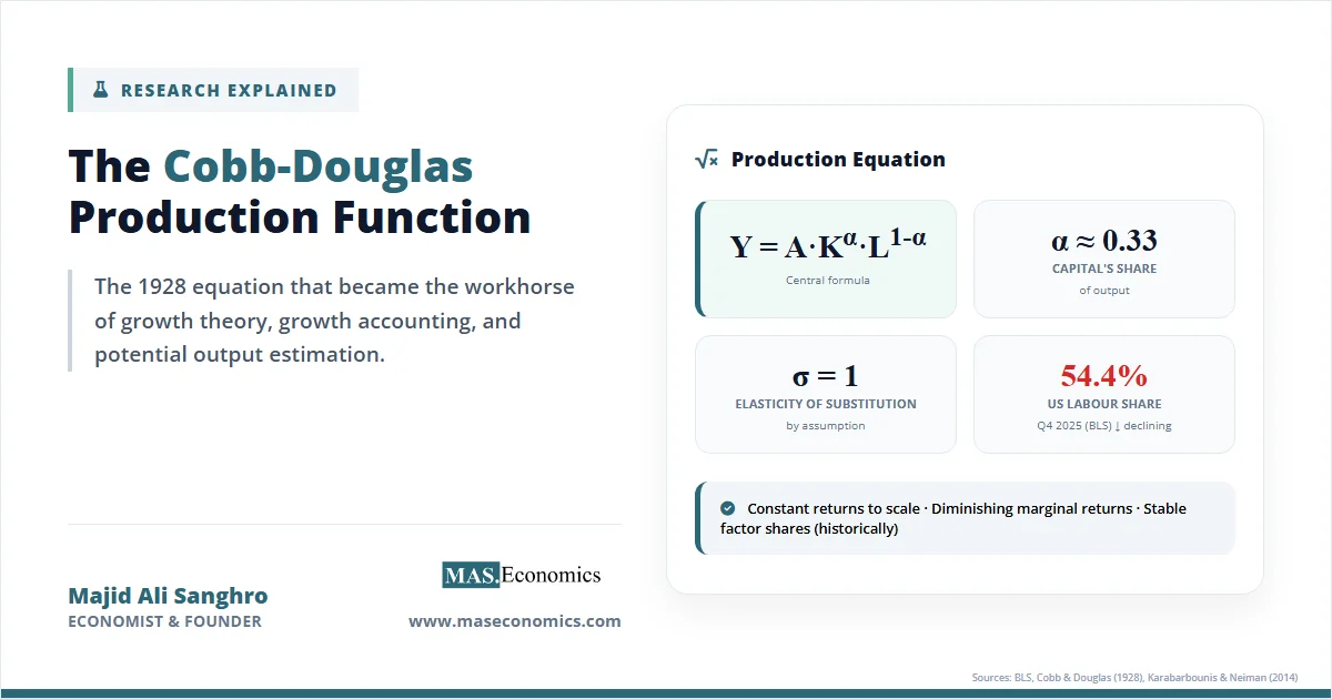
Douglas took the problem to his mathematics colleague Charles Cobb. The question Cobb faced was simple: find a functional form relating output \( Y \) to capital \( K \) and labour \( L \) that (a) fits the data, (b) has economically sensible properties, and (c) is mathematically manageable. The answer he proposed was the multiplicative power function now bearing both their names:
\( Y = A \, K^{\alpha} \, L^{\beta} \)
The beauty of this choice lies in what happens when you take logarithms. A non-linear relationship in levels becomes a linear one in logs, which meant Cobb and Douglas could run a straight-line regression on 1920s-era desk calculators and recover estimates of \( \alpha \) and \( \beta \). When they did the estimation, they found values of roughly 0.25 and 0.75, numbers that closely matched the observed split of US national income between capital and labour. That coincidence, between a free parameter estimated from output data and a moment of the income distribution, was the finding that turned a curve-fitting exercise into a theory of production and distribution.
The function solved the problem Douglas started with: it let him decompose output growth into separate contributions from each factor, plus a residual that would later be named total factor productivity and would itself become one of the most studied quantities in economics. It also planted a deeper claim. If the exponents in the production function really did correspond to the income shares of capital and labour, then the same mathematical object governed both how goods are produced and how the income from producing them is divided. That link, between production technology and distribution, is what makes the Cobb-Douglas function a theory rather than a curve fit.
The Equation in Detail
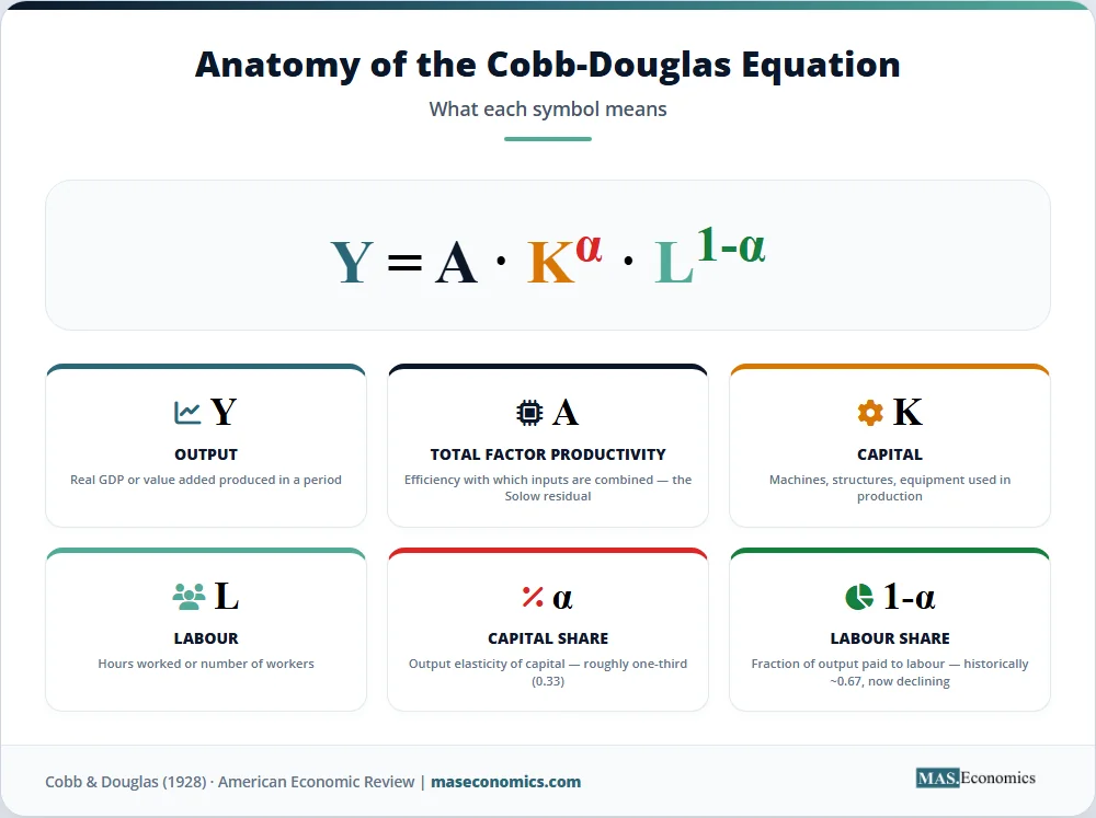
The modern, canonical form of the Cobb-Douglas production function with two factors is:
where \( Y \) is real output, \( K \) is the capital stock, \( L \) is labour input (hours worked or workers employed), \( A \) is total factor productivity, and \( \alpha \in (0,1) \) is the output elasticity of capital. The constraint that the exponents sum to one imposes constant returns to scale, meaning that doubling both inputs doubles output. This is the textbook version, and it is the one embedded in the Solow-Swan growth model and its descendants.
Two properties follow immediately. The marginal product of each factor is:
Both marginal products are positive but declining in their own factor, so the function exhibits diminishing marginal returns along every input dimension. Adding another machine to a fixed stock of workers raises output, but by less than the previous machine did. This is the engine that drives the Solow model toward a steady state.
Under perfect competition, each factor is paid its marginal product. Multiplying through gives the total payment to capital as \( \alpha Y \) and to labour as \( (1-\alpha) Y \). The capital share of income is therefore exactly \( \alpha \), and the labour share is exactly \( 1-\alpha \), regardless of how much capital or labour the economy has. This is the distributional miracle of the Cobb-Douglas form: technology and income distribution are pinned down by a single parameter.
The elasticity of substitution between capital and labour, denoted \( \sigma \), measures how easily one factor can replace the other when their relative prices change. For the Cobb-Douglas function, \( \sigma = 1 \) exactly, a unique feature that distinguishes it from the broader CES (constant elasticity of substitution) family. When \( \sigma = 1 \), a one percent rise in the wage-rental ratio leads to exactly a one percent rise in the capital-labour ratio, and factor shares stay put.
The table below summarises the variables and parameters that appear throughout growth theory, labour economics, and development accounting whenever this function is deployed.
| Symbol | Name | Economic meaning | Typical range or value |
|---|---|---|---|
| \( Y \) | Output | Real value added or GDP produced in a period | Units of real GDP |
| \( K \) | Capital stock | Machines, structures, and equipment used in production | Units of real capital |
| \( L \) | Labour input | Hours worked or employment | Hours or persons |
| \( A \) | Total factor productivity | Efficiency with which inputs are combined; the Solow residual | Index, typically normalised |
| \( \alpha \) | Capital share / output elasticity of capital | Percentage change in output from a one percent rise in capital | 0.30–0.40 in advanced economies |
| \( 1-\alpha \) | Labour share | Fraction of output paid to labour | 0.60–0.70 historically; lower recently |
| \( \sigma \) | Elasticity of substitution | Ease of substituting capital for labour | Exactly 1 by construction |
| \( \text{MP}_K, \text{MP}_L \) | Marginal products | Additional output from one more unit of each factor | Positive, diminishing |

| |||
One more derivation is worth pausing on, because it shows up repeatedly in growth accounting. Taking logs of the production function and differentiating with respect to time gives the growth decomposition:
where \( \hat{X} \) denotes the growth rate of variable \( X \). This equation is the basis of every Solow-style exercise that asks how much of a country’s growth came from capital accumulation, from labour force expansion, and from technological progress. Rearranged, it gives the Solow residual:
which is what economists mean when they say a country’s growth was “mostly TFP” or “mostly factor accumulation.” National income measurement and growth accounting cannot be separated from this decomposition.
What the Function Takes for Granted
Every property that makes the Cobb-Douglas function tractable is also an empirical assumption that may or may not hold. Three of these assumptions deserve particular scrutiny.
Constant returns to scale. The restriction \( \alpha + \beta = 1 \) is usually imposed rather than tested. It rules out increasing returns of the kind emphasised in endogenous growth theory, where spillovers from knowledge or ideas allow aggregate production to scale more than proportionally. When Paul Romer built his models of idea-driven growth in the 1980s and 1990s, the departure from constant returns at the aggregate level was the whole point.
Unit elasticity of substitution. The Cobb-Douglas function forces \( \sigma = 1 \). Empirical estimates of the aggregate elasticity of substitution typically fall in the range of 0.4 to 0.9 for advanced economies, significantly below one. When \( \sigma < 1 \), capital and labour are gross complements rather than substitutes, and factor shares are no longer constant. This matters because, if the true elasticity is below one, then falling prices of capital goods should increase rather than decrease the labour share, the opposite of what the data show.
Constant factor shares. A direct implication of Cobb-Douglas is that the share of national income accruing to labour should be constant over time. For most of the twentieth century, this seemed approximately true, which is one of Nicholas Kaldor’s famous stylised facts of growth. But Loukas Karabarbounis and Brent Neiman’s 2014 paper in the Quarterly Journal of Economics documented that the global labour share has declined significantly since the early 1980s across the large majority of countries and industries. US Bureau of Labor Statistics data shows the nonfarm business labour share was 54.4 percent in the fourth quarter of 2025, well below the 63–65 percent levels that prevailed in the 1960s and 1970s. If factor shares are moving, the Cobb-Douglas assumption of constancy is wrong at exactly the frequency that matters for long-run growth.
A fourth concern is subtler and has been raised repeatedly since the 1970s. Anwar Shaikh and others have argued that the Cobb-Douglas function is not really a theory of production at all, but an accounting identity in disguise. If factor shares are stable in the data and one regresses output on capital and labour, the resulting equation must look Cobb-Douglas regardless of the true underlying technology, because the exponents are pinned down by the shares rather than by any causal relationship. This “Humbug production function” critique does not prove the Cobb-Douglas form is wrong, but it shows that its apparent empirical success does not confirm as much as one might think.
Does the Data Actually Say It Holds?
The evidence on the Cobb-Douglas function has accumulated in layers. The first layer is the one Cobb and Douglas themselves provided: for US manufacturing between 1899 and 1922, the estimated exponents matched the observed factor shares, and the function fit the data with a high R-squared. Subsequent studies on different countries, industries, and time periods repeatedly found similar results, and by the 1950s the function was standard in empirical work.
The second layer is the critique from the elasticity-of-substitution literature. Once the CES production function was introduced in 1961 by Arrow, Chenery, Minhas, and Solow, economists had a benchmark against which Cobb-Douglas could be formally tested. The test is a restriction: Cobb-Douglas is the special case of CES where \( \sigma = 1 \). A Congressional Budget Office survey of these studies found estimates of \( \sigma \) ranging from 0.32 to 1.16, with most significantly below unity. Taken at face value, this evidence rejects Cobb-Douglas in favour of a more flexible CES specification.
The third layer is the factor-shares evidence already mentioned. The combination of declining labour shares and persistent cross-sectional dispersion in capital-labour ratios across firms and industries is hard to square with a production function that forces shares to be equal to constant exponents.
The chart below illustrates the core mechanics of the function that any empirical critique has to contend with. It shows output \( Y \) as labour \( L \) varies, for three fixed levels of the capital stock, holding productivity \( A \) constant. The curves are concave, reflecting diminishing returns to labour, and they shift up as capital rises, reflecting capital-labour complementarity.
Figure 1. Output as a function of labour input, under a Cobb-Douglas production function with \( \alpha = 0.33 \), for three levels of capital stock. Source: author’s calculations using the standard two-factor Cobb-Douglas specification.
The concavity of each curve is the visual expression of diminishing marginal returns. The vertical gap between the curves at any given labour level reflects the contribution of the capital stock to total output, and the fact that this gap grows slowly (because \( \alpha = 0.33 \)) mirrors the stylised fact that capital’s share is roughly one-third of income in advanced economies.
The empirical verdict, then, is mixed and depends on what one is asking. As a literal description of how firms combine inputs, the Cobb-Douglas function is probably wrong. As a summary of the long-run comovement between aggregate output, capital, and labour in advanced economies, it fits surprisingly well. And as a tractable closed-form approximation for models that need to produce sensible comparative statics and balanced-growth paths, it remains unbeatable. The function survives not because it is right, but because its errors are usually small enough to ignore at the level of aggregation where macroeconomists typically work.
From Blackboard to Policy
The Cobb-Douglas function’s influence extends far beyond the original 1928 paper because it is the building block of almost every modern growth model. The Solow-Swan model uses it to derive the convergence properties of capital accumulation and to show that long-run per-capita growth must come from technological progress rather than saving. Endogenous growth models, from Romer’s 1990 ideas-based framework to the Aghion-Howitt Schumpeterian model, layer additional structure on top of a Cobb-Douglas core. Dynamic stochastic general equilibrium (DSGE) models used at central banks, including the Federal Reserve’s FRB/US model, the Bank of England’s COMPASS, and the European Central Bank’s Smets-Wouters framework, rely on Cobb-Douglas production blocks for their supply side. When economists speak of potential output, they are usually referring to the output level implied by a Cobb-Douglas production function evaluated at full-employment inputs.
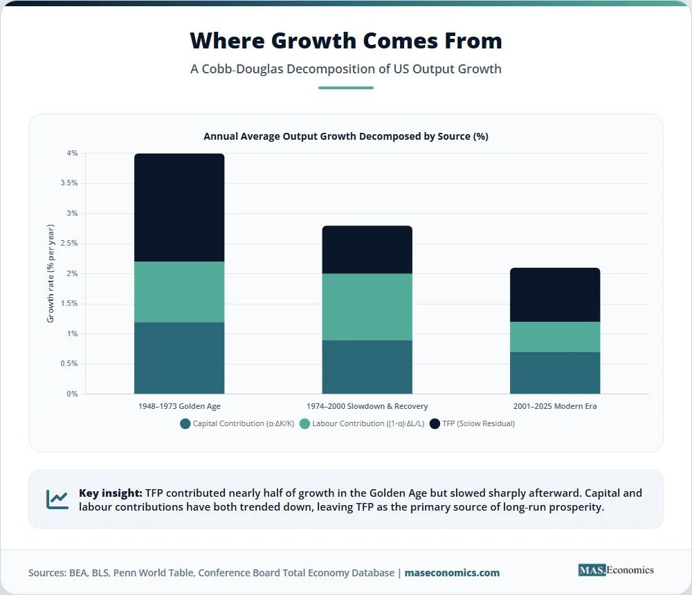
The function is equally embedded in development and growth accounting. The Conference Board’s Total Economy Database, the Penn World Table, and the IMF’s country-level growth decompositions all use Cobb-Douglas technology to separate output growth into contributions from capital deepening, labour input, and TFP. When the Congressional Budget Office or the OECD publishes a projection of long-run US or European growth, the number is typically generated from a Cobb-Douglas framework with assumptions about future labour force participation, investment rates, and productivity trends. Getting these projections roughly right matters for fiscal policy, retirement system solvency, and debt sustainability calculations that run decades into the future.
In labour economics, the Cobb-Douglas function underlies the standard derivation of factor demand curves. The result that wages equal the marginal product of labour, combined with the Cobb-Douglas marginal product expression, gives labour demand curves that decline in the wage and shift with capital and technology. This is the framework used to estimate the effects of automation, immigration, and minimum wages on employment, and it is the baseline against which more flexible specifications are tested.
In policy debates, the structure of the Cobb-Douglas function shapes what economists believe is possible. If the function holds, then permanent subsidies to investment raise the capital-output ratio but do not change the long-run growth rate, which is driven solely by TFP. This implication, developed rigorously in the Solow model, is why economists are often sceptical of industrial policy aimed at raising investment unless it is accompanied by a story about technology or knowledge spillovers. By contrast, if the true production function has increasing returns or knowledge externalities, as endogenous growth theorists argue, then the policy space opens up considerably. The 2024 Nobel Prize awarded to Daron Acemoglu, Simon Johnson, and James Robinson for work on institutions and growth sits partly in the tradition of challenging the simple Cobb-Douglas view.
The function also quietly shapes how we think about current debates. Concerns about AI and productivity are typically framed as a question about whether the technology will show up as a shift in \( A \) or as a change in the effective capital stock. Debates about the declining labour share are debates about whether \( 1-\alpha \) is still constant. Discussions of automation and inequality depend on whether the elasticity of substitution between capital and labour is above or below one, a question the Cobb-Douglas function settles by assumption but that matters enormously for the distributional consequences of technological change. In each case, the language and intuitions come from an equation written nearly a century ago to describe US manufacturing.
What has kept the function alive is not empirical triumph but analytical indispensability. Economists writing down a new model still reach for Cobb-Douglas first because it produces closed-form solutions, because it is consistent with balanced growth, and because its parameters have immediate economic interpretations. When the question being asked does not depend on the elasticity of substitution or the behaviour of factor shares, the function’s restrictions are harmless. When it does, economists reach for CES or translog alternatives, but they usually report Cobb-Douglas results alongside as a benchmark.
MASEconomics Explains
Four economic concepts behind the Cobb-Douglas production function
Conclusion
The Cobb-Douglas production function began as a curve-fitting exercise on 1920s US manufacturing data and grew into the default production technology of modern macroeconomics. Its assumptions of constant returns to scale, unit elasticity of substitution, and stable factor shares have all been challenged by evidence, most notably by the documented decline in the global labour share since the early 1980s and by estimates of the elasticity of substitution that fall below one. Yet the function endures because its closed-form tractability, interpretable parameters, and compatibility with balanced growth make it the indispensable first approximation. Every central bank projection of potential output, every growth accounting exercise, and every textbook derivation of the steady state rests on the same equation Cobb and Douglas wrote down in 1928. The Cobb-Douglas production function is wrong in specific, measurable ways, but it is wrong in ways macroeconomists have learned to work around, which is why it remains the equation behind nearly every growth model.
Did you find this article helpful? Share it with someone who loves economics. And remember, at MASEconomics, we make complex ideas simple.