When the Bill and Melinda Gates Foundation announced in 2020 that it would invest over $1.6 billion in Gavi to support childhood vaccination in low‑income countries, the underlying economics was straightforward. A vaccinated child does not just gain personal immunity. Their neighbors, classmates, and unvaccinated relatives also become less likely to catch the disease. The private benefit to the family is real, but only a fraction of the social benefit. When private decisions are made on the basis of private benefits alone, the market produces too few vaccinations, too little education, and too little basic research relative to what society would choose if every spillover were priced. The positive externality diagram shows exactly how that gap arises and how a subsidy equal to the marginal external benefit can close it.
Positive externalities are the mirror image of the negative case. Private benefits understate social benefits, the market underproduces relative to the social optimum, and a per‑unit subsidy set at the marginal external benefit shifts the effective demand curve upward to coincide with the social benefit curve. The geometry is small, but it underwrites several centuries of policy thinking on education, public health, and innovation.
Spillover Benefits and Private Decisions
A positive externality exists whenever a private transaction generates value for parties who are not part of the deal and who pay nothing for it. Vaccination is the canonical example. The vaccinated person reduces their own infection probability and also reduces the probability that they pass the disease on to others. The private buyer captures the first benefit through their own willingness to pay. The second benefit, called the marginal external benefit (MEB), flows to third parties who do not enter the demand curve.
Education works the same way. A graduate captures private returns through higher wages, but society also gains through more productive coworkers, lower crime, better-informed voting, and faster knowledge diffusion. Basic scientific research generates spillovers that are notoriously hard to capture privately: a 1962 paper by Kenneth Arrow on the economics of invention argued that this is precisely why private firms underinvest in fundamental research relative to the social optimum. Restoration of historic buildings, beekeeping, residential solar panels, and even routine flu shots all share the same structural feature. The decision-maker sees one curve. Society sees a higher one.
The analysis in this article focuses on the consumption case, where the spillover sits on the demand side. Marginal private cost equals marginal social cost because production itself imposes no third-party harm. The standard supply curve is therefore both the MPC and the MSC. The divergence is between marginal private benefit (MPB), which is the standard demand curve, and marginal social benefit (MSB), which sits above MPB by the marginal external benefit at every quantity.
The Underproduction Diagram
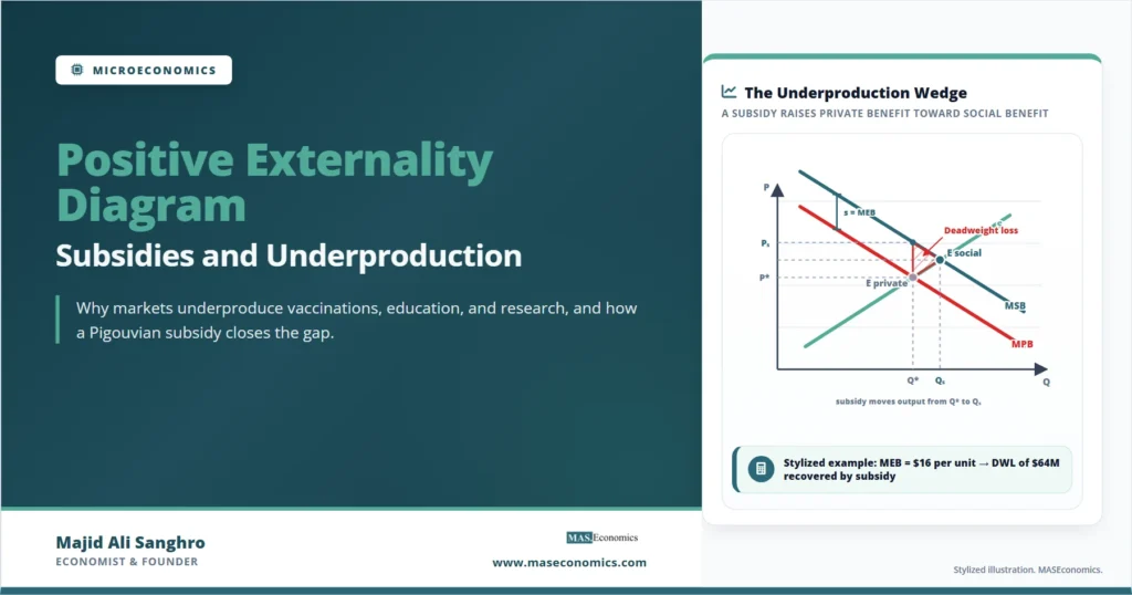
The figure below shows the market for a good with a positive consumption externality. MPB is the standard demand curve, sloping downward as private willingness to pay falls with quantity. MSB sits above MPB by the marginal external benefit. Supply, which equals MSC, slopes upward in the usual way. The private market clears at Q* where supply meets MPB. The socially efficient quantity sits at Qs where supply meets MSB. Because MSB is higher than MPB at every quantity, Qs is to the right of Q*. The market underproduces.

The geometry is the mirror image of the negative externality case. There, the wedge sat between MPC and MSC on the cost side, and the market overproduced. Here, the wedge sits between MPB and MSB on the benefit side, and the market underproduces. In both cases, the welfare loss is a triangle, but the triangle now opens to the right with its apex at E social on the right and its vertical base at Q* on the left. The base height is the MEB at the private quantity, and the base width is the gap between Qs and Q*.
The Corrective Subsidy
A per-unit subsidy equal to MEB at Qs corrects the externality. The subsidy can be paid to either side of the market without changing the welfare result. If paid to consumers, the effective demand curve they face shifts upward to coincide with MSB. If paid to producers, the effective supply curve shifts downward by the same amount. In both cases, the market trades at Qs, the quantity society wants. The diagram below shows the case where the subsidy is paid to producers, which simplifies the visual.
Pigouvian Subsidy Rule
Take the same stylized market: inverse demand (MPB) P = 100 − Q, supply (MSC) P = 20 + Q, and a constant marginal external benefit MEB = $16, so MSB = 116 − Q. Quantities are in millions of units, prices in dollars.
Without the subsidy, the market equilibrates at Q* = 40 and P* = 60. Society’s preferred quantity is Qs, where MSB meets supply: 116 − Q = 20 + Q gives Qs = 48. At Qs, supply gives a producer price of 68, and MPB gives a consumer willingness to pay of 52. The subsidies = 16 bridges this gap. Consumers pay 52 out of pocket; producers receive 68, with the government paying the 16-per-unit subsidy. The subsidy cost is s × Qs = 16 × 48 = $768 million.
The welfare gain is the original deadweight loss recovered. The triangle base is Qs − Q* = 8, and its height is MEB = 16, giving an area ½ × 8 × 16 = $64 million. That is the value society leaves on the table when the externality is ignored.
| Component | No Subsidy (Q* = 40) | Optimal Subsidy (Qs = 48) | Change |
|---|---|---|---|
| Consumer Surplus | 800 | 1,152 | +352 |
| Producer Surplus | 800 | 1,152 | +352 |
| External Benefits Realized | 640 | 768 | +128 |
| Subsidy Cost | 0 | −768 | −768 |
| Total Social Surplus | 2,240 | 2,304 | +64 |
| Externality DWL | 64 | 0 | −64 |
|
Source: Stylized example based on standard formulas.
|
|||
The accounting has a feature that surprises some readers. Consumer and producer surplus both rise substantially. External benefits realized also rise. The subsidy cost is high in absolute terms, but the welfare gain is positive once all four components are netted. The subsidy transfers from taxpayers (who fund it) to the parties involved in the transaction, and the externality correction creates new value worth exactly the DWL triangle. The transfer is not part of the welfare gain. The recovered triangle is.
The Pigouvian subsidy and the Pigouvian tax are formal mirrors but practical opposites. A tax shrinks output and raises revenue. A subsidy expands output and costs revenue. The welfare gain in both cases equals the externality deadweight loss recovered. Whether a country can afford the subsidy depends on its fiscal position, which is part of why positive externalities are often corrected through public provision, mandates, or tax credits rather than direct per-unit payments.
Where Positive Externality Subsidies Show Up in Practice
The diagram has guided several decades of policy in three large areas. Childhood vaccination is the clearest case. Most high-income countries provide childhood vaccines free at the point of use, fully internalizing the herd-immunity externality through a 100 percent public subsidy. The World Health Organization tracks global immunization coverage by antigen, and the cross-country variation in coverage rates closely follows the degree of public subsidy and accessibility. Where governments rely on private payment, coverage falls below the social optimum.
Education subsidies follow the same logic. Compulsory schooling, free public education through secondary level, and means-tested higher-education grants are partial subsidies that compensate for the gap between private and social returns to schooling. A long literature in labor economics, including work by James Heckman and others on early childhood education, has tried to estimate the social rate of return. The estimates vary, but they consistently exceed the private rate, which is the structural justification for public funding.
Research and development subsidies, R&D tax credits, and patent systems address the third major case. Patents are an indirect subsidy: they grant temporary monopoly profits to inventors, raising private returns toward the social return for a limited period. Direct R&D grants and tax credits do the same thing more transparently. The US R&D tax credit, the EU Horizon programs, and the basic-science budgets of national laboratories are all institutional answers to the question: how much should government pay to close the gap between private and social returns on research? The diagram does not give a number, but it gives the shape.
Less obvious cases include solar panel installations, energy-efficiency retrofits, and electric vehicle adoption. Each generates climate benefits that the private buyer does not fully capture, which is the justification for the per-unit subsidies that most major economies offer for these technologies. The diagram in this article applies directly to each case, with MEB representing avoided climate damages, avoided local pollution, or accelerated technology spillovers.
Limitations of the Subsidy Diagram
The picture is clean, but its assumptions matter. Four are worth pulling out.
Real MEB is rarely constant. Vaccination spillovers are largest at low coverage rates and shrink as coverage approaches herd immunity. The marginal social benefit curve in real settings is steeper than MPB in some quantity ranges and flatter in others. A constant per-unit subsidy is therefore a second-best approximation. Real-world policy often combines a per-unit subsidy with a mandate or with progressive payment structures to capture the curvature.
The subsidy must reach the right margin. A subsidy paid to college tuition raises the demand for college but may not raise enrollment by people on the relevant margin if those people are also constrained by liquidity, information, or readiness. Targeted interventions for at-risk students often outperform broad tuition subsidies in cost-effectiveness terms, even though the broad subsidy is what the diagram naively recommends.
Subsidies are funded through taxes that themselves carry deadweight loss. The welfare arithmetic above assumes the subsidy is funded from a lump-sum tax that creates no distortion. Real funding sources are distortionary income or consumption taxes, which means the true welfare gain from a Pigouvian subsidy is smaller than the diagram suggests. The shadow cost of public funds enters as an additional consideration in serious applied work.
Finally, government failure can be as costly as market failure. Subsidy programs can be captured by incumbent producers, mistargeted, or hard to phase out once installed. The political economy of subsidies is its own large literature, much of it tracing back to the public-choice analysis of how interventions designed to correct one inefficiency can create others. The diagram identifies the first-best policy. Whether the first-best policy is implementable is a separate question.
Explains
Three concepts behind the underproduction wedge
From the subsidy diagram to the broader logic of welfare-correcting policy and public economics.
Explore the MASEconomics BlogConclusion
The positive externality diagram is the mirror image of the negative case. Marginal private benefit lies below marginal social benefit, the private market equilibrium produces less than the social optimum, and the foregone surplus on the units that go unproduced is the deadweight loss the externality creates. A per‑unit subsidy set equal to the marginal external benefit closes the gap. The effective demand curve shifts to MSB, the market trades at Qs, consumer prices fall, producer prices rise, and the welfare triangle that would otherwise be lost is recovered. The arithmetic is straightforward; the geometric symmetry with the tax case is exact.
The diagram does not answer every question in education, public health, or innovation policy. Real damage and benefit functions are nonlinear, real markets carry multiple distortions, and real subsidies are funded through taxes that create their own welfare costs. What the diagram does is identify the target: shift output toward the quantity where social benefit equals social cost. Half a century of vaccination programs, education subsidies, R&D tax credits, and clean energy incentives has been an extended attempt to apply this small piece of geometry to real policy. The successes and failures of those programs map onto the diagram’s strengths and limits in ways that should now be visible.
Frequently Asked Questions
What is a positive externality?
A positive externality is a benefit generated by a transaction that flows to third parties who are not part of the transaction and do not pay for it. Vaccination, education, basic research, beekeeping, and historic-building restoration are all standard examples. The decision-maker captures only the private benefit and ignores the spillover, leading to underproduction relative to the social optimum.
How does a subsidy correct a positive externality?
A per-unit subsidy equal to the marginal external benefit shifts the effective demand or supply curve, depending on which side it is paid to. In both cases the market clears at the socially efficient quantity. The consumer pays a lower out-of-pocket price, the producer receives a higher price, and the government covers the difference. The welfare gain equals the externality deadweight loss that the unregulated market would have left on the table.
Why does the market underproduce in the positive externality case?
Because private buyers set quantity where supply meets their private willingness to pay, ignoring the additional benefit that spills over to others. The socially efficient quantity is determined by supply meeting marginal social benefit, which is higher than marginal private benefit at every quantity. The gap between the two quantities is the source of the deadweight loss triangle.
Does it matter whether the subsidy is paid to consumers or producers?
For the welfare result, no. In both cases the market trades at the socially efficient quantity, the same total subsidy is paid, and the same welfare triangle is recovered. The split of the gain between consumer surplus and producer surplus depends on the relative elasticities of demand and supply, but total surplus and total subsidy cost are identical either way.
Why are vaccinations and education funded through subsidies rather than left to the market?
Because the social benefits of vaccination and education extend well beyond the private benefits captured by the individual. Herd immunity, lower disease transmission, more productive coworkers, lower crime rates, and faster knowledge diffusion are all spillovers that private buyers do not pay for. A subsidy or, in the limit, free public provision raises consumption toward the socially efficient level.
Can a positive externality subsidy fail?
Yes, in several ways. The subsidy may not reach the relevant margin if the underlying barrier is information or liquidity rather than price. The funding source may carry its own distortions. The program may be captured by incumbent producers or used inefficiently. And the marginal external benefit may be miscalibrated, leading to over- or under-subsidization. The diagram identifies the first-best policy; implementation is a separate problem.
Thanks for reading! If you found this helpful, share it with friends and spread the knowledge. Happy learning with MASEconomics