Sacrifice Ratio: Output Cost of Disinflation

Between October 1979 and August 1982, the Federal Reserve under Paul Volcker raised the federal funds rate to roughly 19 percent. US unemployment climbed from 6 percent to 10.8 percent, real GDP contracted across two formal recessions, and CPI inflation fell from about 13 percent to under 4 percent. The cost of that disinflation, measured in lost output, became the canonical reference point for a concept central banks have argued about ever since. The sacrifice ratio asks a simple question with no simple answer: how much output must an economy give up to bring inflation down by one percentage point? Estimates range from below one to above five, depending on the country, the episode, and the assumptions of the researcher. The dispersion is not a measurement problem. It is the empirical record of how much disinflation costs depend on credibility, expectations, and the speed at which policy moves.

Measuring the Sacrifice Ratio

The sacrifice ratio is defined as the cumulative loss of output, expressed as a share of trend or potential GDP, divided by the cumulative reduction in trend inflation over the same disinflation episode. The basic formula is straightforward:

\( y^{*}_{t} – y_{t} \) is the output gap in period \( t \), accumulated from the start of the disinflation \( t=0 \) to its conclusion \( T \). The denominator is the change in trend inflation over the same window. The ratio is reported in units of percent of GDP per percentage point of inflation reduction.

A sacrifice ratio of two means an economy lost a cumulative 2 percent of GDP for every percentage point of inflation reduction. A sacrifice ratio of zero would mean inflation fell without any output cost, a “costless” or “credible” disinflation. The empirical literature has produced estimates across most of that range. Laurence Ball’s influential 1994 NBER study, “What Determines the Sacrifice Ratio?”, identified 65 disinflation episodes across nine OECD economies between 1960 and 1991 and found a median sacrifice ratio of around 1.5, with substantial variation across countries and episodes.

The intuition behind the cost is the Phillips curve trade-off. When a central bank tightens policy to reduce inflation, it raises real interest rates above their neutral level. Investment and interest-sensitive consumption fall. Aggregate demand drops below potential output. Unemployment rises. As the Phillips curve framework predicts, slack in the labor market eventually feeds into slower wage growth, slower price increases, and lower inflation. The output gap closes only after inflation has come down, which is why the sacrifice ratio integrates losses over the full episode rather than measuring them at a single point in time.

Costly and Costless Disinflation

Two opposing theoretical traditions frame the debate. The adaptive expectations view, dominant before the late 1970s, treated expected inflation as a function of past inflation. Under that assumption, disinflation requires an extended period of below-potential output to grind down expected inflation gradually. The sacrifice ratio is large and largely unavoidable. The textbook expectations-augmented Phillips curve makes this explicit:

Inflation \( \pi_{t} \) depends on expected inflation \( \pi^{e}_{t} \), the unemployment gap \( (u_{t} – u^{*}) \) scaled by sensitivity \( \alpha \), and a supply-shock term \( \varepsilon_{t} \). Disinflation requires either a fall in \( \pi^{e}_{t} \) or a sustained positive unemployment gap.

The rational expectations critique, developed in the 1970s by Robert Lucas, Thomas Sargent, and others, challenged that conclusion. If the public understands the central bank’s policy rule and believes the policymaker is committed to reducing inflation, expected inflation should adjust immediately to the announced target. In that case, no sustained unemployment gap is required, and the sacrifice ratio can approach zero. Sargent’s 1982 paper, “The Ends of Four Big Inflations”, examined the post-World War I European hyperinflations and argued that credible regime changes ended inflation rapidly without prolonged recession. The keyword in that finding is “credible.” Without credibility, the rational expectations result does not hold, and the sacrifice ratio reverts to the adaptive case.

In practice, neither extreme describes most disinflations. The empirical literature finds positive but variable sacrifice ratios, which is consistent with expectations that are partly forward-looking, partly backward-looking, and sensitive to the specific policy framework in place.

Volcker, Thatcher, and the High-Cost Cases

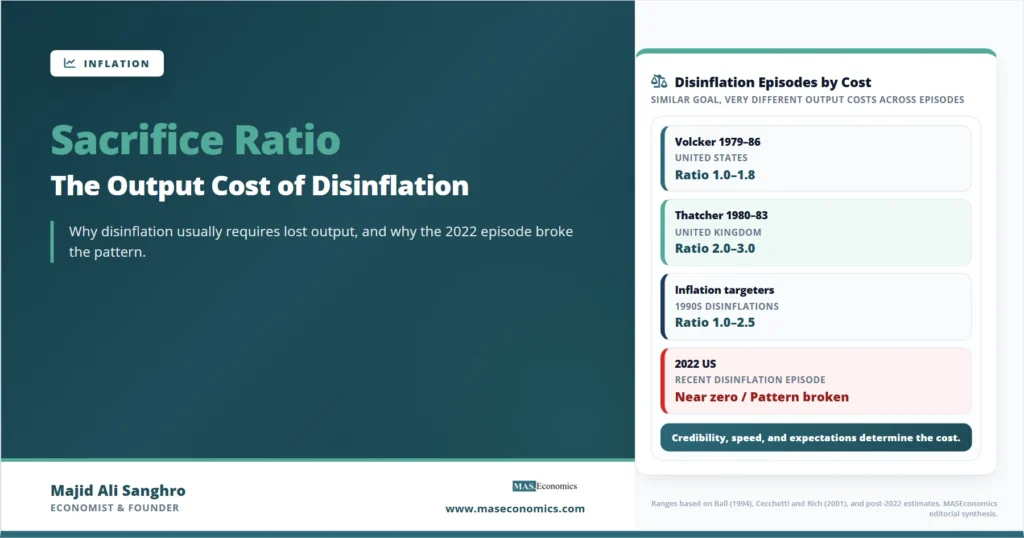
The Volcker disinflation in the United States is the most studied disinflation episode in the literature. The cumulative output gap from 1979 to 1986 has been estimated at between 10 and 16 percent of GDP, depending on the trend specification, against an inflation reduction of about 9 percentage points. The implied sacrifice ratio sits in the range of 1.0 to 1.8 by most standard calculations, broadly consistent with Ball’s later cross-country median. The cost was concentrated in the 1981–1982 recession, the deepest US downturn between the Great Depression and the 2008 financial crisis. As stagflation data from that period shows, the inflation reduction came alongside double-digit unemployment.

The Thatcher disinflation in the United Kingdom produced similar arithmetic. UK CPI inflation fell from roughly 18 percent in 1980 to 5 percent by 1983, and the cumulative output loss measured against potential GDP was substantial, with manufacturing employment falling by more than 20 percent. Estimates of the UK sacrifice ratio for that episode cluster around 2 to 3, somewhat above the US figure, reflecting the deeper recession in the industrial sector.

Ball’s classification of episodes pointed to three factors that explained the cross-country variation. Faster disinflations had lower sacrifice ratios than slower ones, a finding that pushed back against the gradualist orthodoxy of the 1970s. Countries with more flexible labor markets and less nominal wage rigidity had lower sacrifice ratios. And countries with more credible monetary frameworks had lower ratios because expectations adjusted more quickly.

Table 1. Sacrifice Ratio Estimates for Major Disinflation Episodes

Episode	Country	Period	Inflation Reduction	Sacrifice Ratio (est.)
Volcker disinflation	United States	1979–1986	~9 pp	1.0–1.8
Thatcher disinflation	United Kingdom	1980–1983	~13 pp	2.0–3.0
Bundesbank disinflation	West Germany	1980–1986	~4 pp	2.0–3.5
Inflation targeting adoption	Canada	1991–1993	~4 pp	1.5–2.5
Inflation targeting adoption	New Zealand	1989–1992	~6 pp	1.0–2.0
2022 disinflation	United States	2022–2024	~6 pp	near zero (so far)
OECD median, 1960–1991	Nine economies	65 episodes	varies	~1.5
Source: Ball (1994), NBER WP 4306; Cecchetti and Rich (2001); Gordon and King (1982); Federal Reserve and BLS data; BIS Annual Economic Report 2023. Estimates reflect mid-range published values; methodological choices affect levels.

Disinflation Speed and Sacrifice

One of the most policy-relevant findings in the sacrifice-ratio literature concerns the speed of disinflation. The pre-Volcker consensus, often called gradualism, held that bringing inflation down slowly would minimize the output cost by giving wages and prices time to adjust. Ball’s cross-country evidence overturned that view. Faster disinflations were associated with lower, not higher, sacrifice ratios. The mechanism is credibility: a rapid, decisive policy move signals that the central bank is willing to absorb short-run costs, which speeds the adjustment of inflation expectations and shortens the period of below-potential output.

The “cold turkey” approach pursued by Volcker, in which the federal funds rate was raised aggressively and sustained at levels far above measured inflation, fits this pattern. The disinflation was painful but compressed. Episodes where central banks tightened slowly tended to produce longer periods of below-potential output without achieving inflation reduction any faster.

The Disinflation Trade-Off: Output Gap and Inflation

Stylized illustration. Inflation falls above the zero line; the output gap opens below the zero line. The shaded area is the cumulative output loss that enters the sacrifice ratio numerator.

Credibility and the Sacrifice Ratio

Ball’s empirical work and a substantial follow-up literature pointed to credibility as the most powerful determinant of the sacrifice ratio. The intuition runs through expectations. If households, firms, and wage-setters believe inflation will fall, they will set prices and wages consistent with lower inflation, which reduces the need for a sustained output gap. If they do not believe the central bank, they will continue to set wages and prices based on past inflation, and the only way to bring inflation down is to force it down through demand compression.

This is why inflation targeting reduces sacrifice ratios in the long run. The framework makes the central bank’s objective transparent, gives the public a focal point for expectations, and builds reputation over successive episodes. The countries that adopted inflation targeting in the early 1990s, including New Zealand (1989), Canada (1991), the United Kingdom (1992), and Sweden (1993), generally experienced lower sacrifice ratios in subsequent disinflations than they had in the 1970s and 1980s.

The other side of credibility is the Friedman-Phelps natural rate hypothesis. In the long run, there is no trade-off between inflation and unemployment because expectations fully adjust to the inflation rate that policy delivers. The sacrifice ratio is therefore a short-run concept. The output cost is paid during the transition; once the new equilibrium is reached, unemployment returns to its natural rate at the lower inflation rate. What credibility changes is the length and depth of that transition.

Near-Zero Sacrifice Ratio of 2022–2024

The recent US disinflation has emerged as a striking outlier in the historical record. Between June 2022 and late 2024, US headline CPI inflation fell from 9.1 percent to roughly 3 percent, a reduction of about 6 percentage points. Over the same period, the unemployment rate rose modestly from around 3.6 percent to 4.1 percent, and real GDP continued to grow. There was no recession. The cumulative output gap over the episode was small or arguably zero, depending on how potential output is measured. The implied sacrifice ratio is close to zero.

This outcome was not predicted by standard models. In late 2022, the Federal Reserve Bank of New York’s Survey of Professional Forecasters and most private-sector forecasts saw a recession as likely. Larry Summers and several others argued publicly that unemployment would need to rise to 5 percent or more for several years to bring inflation back to target. None of that happened. The puzzle has spawned an active literature with several candidate explanations.

The first explanation is supply normalization. As the 2022–23 global inflation surge showed, much of the inflation peak reflected pandemic supply-chain disruptions and the Russian invasion of Ukraine. When supply chains normalized and energy prices retreated, headline inflation fell mechanically without any contribution from demand compression. The second is anchored expectations. Long-run inflation expectations from the New York Fed and Michigan surveys stayed near 3 percent throughout the episode, which meant that wage and price setters did not require a recession to convince them that inflation would return to target. The third is labor-market structure: most of the labor-market normalization came through declines in job openings rather than increases in unemployment, which kept the output gap small while still cooling wage pressure. Bernanke and Blanchard’s NBER working paper on pandemic-era inflation supported the supply-side reading, attributing most of the inflation rise and most of the subsequent decline to product-market shocks.

Whether the 2022–2024 sacrifice ratio belongs in the historical comparison set is itself disputed. Several authors have argued that the disinflation is incomplete and that the final mile, from 3 percent to 2 percent, could yet require a more conventional sacrifice. Others argue that the episode demonstrates the cumulative payoff of forty years of credibility investment by the Federal Reserve. The historical record from Ball onward suggests both views could be partly right. Credibility lowers the average sacrifice ratio but does not eliminate the variance across episodes.

Determinants of Estimate Variation

Three measurement issues account for most of the disagreement about how to compute and compare sacrifice ratios. The first is the definition of potential output. The HP filter, linear trend, production function, and CBO output gap series can produce gaps that differ by 2 to 3 percentage points of GDP for the same year, which scales directly into the numerator of the ratio. The second is the choice of inflation measure. Headline CPI, core CPI, PCE, and the GDP deflator behave differently during disinflations, particularly when energy prices contribute to the headline path. The third is episode dating. Where does a disinflation begin and end? Different conventions can change the sacrifice ratio substantially by including or excluding quarters of recovery or persistence.

These choices are not innocent. The same dataset can support claims that disinflation was costly or relatively painless, depending on how the analyst treats potential output and the inflation measure. A useful discipline is to report sacrifice ratios as ranges across reasonable specifications rather than single-point estimates. Ball did this in his original work, and the practice has continued in the IMF and BIS literature.

Limitations of the Sacrifice Ratio

Three limits on the concept are worth marking. First, the sacrifice ratio measures average cost across the transition; it does not measure the distributional incidence of that cost. The Volcker disinflation imposed unemployment disproportionately on manufacturing workers, on Black workers, and on younger workers. Two disinflations with the same sacrifice ratio can have very different welfare implications depending on how the lost output is distributed. Second, the ratio is silent on the gains from lower inflation. A disinflation that costs 2 percent of GDP on the transition path may still be welfare-improving if it durably anchors expectations and reduces future inflation volatility. The standard literature treats this gain as positive but does not quantify it within the sacrifice-ratio framework. Third, the sacrifice ratio assumes a clean separation between supply and demand shocks, which the 2022 experience showed is harder to maintain in practice. When inflation rises for supply-side reasons, a central bank that responds with demand compression is paying a sacrifice ratio that the underlying inflation may not have required.

Explains

Conclusion

The sacrifice ratio remains one of the most useful organizing concepts in monetary policy analysis because it forces an explicit accounting of what disinflation costs and how those costs depend on expectations, credibility, and the speed of policy action. The historical record is clear about three things. Disinflations are usually costly, with the typical OECD episode producing a sacrifice ratio between one and three. Faster disinflations and more credible monetary frameworks reduce that cost, sometimes substantially. And the dispersion of estimates across episodes is large enough that no single number can summarize the relationship between output and inflation.

The 2022–2024 US disinflation has reopened the debate by producing a sacrifice ratio close to zero, which the historical record suggested was rare but possible under specific conditions: supply-driven inflation that reversed mechanically, anchored long-run expectations, and a credible policy framework that did not need to demonstrate commitment because forty years of prior tightening cycles had already done so. Whether that combination represents a new normal or a particular configuration that will not be repeated is the open question. The sacrifice ratio framework helps name the variables that determine the answer, even if it cannot predict the answer in advance.

Frequently Asked Questions

Thanks for reading! If you found this helpful, share it with friends and spread the knowledge. Happy learning with MASEconomics