In 1976, Robert Lucas published a short paper that derailed a generation of macroeconometric forecasting. His argument was deceptively simple. Statistical models estimated on historical data, he wrote, cannot reliably predict what will happen if policy changes, because the parameters of those models are themselves functions of the policy regime that produced the data. Change the regime, and the parameters change. Apply the old coefficients to the new policy, and the forecast is wrong. This argument is the Lucas critique, and inflation modeling has been the field where it has done the most damage to confident empirical claims. The Phillips Curve estimated on 1960s data did not survive the 1970s. The inflation persistence estimated on the 1970s data did not survive the 1980s. The flat Phillips Curve estimated on 2000s data did not survive 2022. Each of these episodes was, in the Lucas critique’s strict sense, a consequence of treating regime-dependent parameters as if they were structural.
Core Argument of the Lucas Critique
The Lucas critique, set out in “Econometric Policy Evaluation: A Critique” (Lucas, 1976), distinguishes two kinds of model parameters. Some parameters describe the underlying preferences and technology of households and firms; these are deep, structural, and policy-invariant. Other parameters describe the reduced-form relationships that economists observe in data; these are policy-dependent because they bundle together structural behavior with the way agents have learned to respond to the prevailing policy rule. When the policy rule changes, the reduced-form parameters shift, even though the underlying preferences and technology have not.
The simplest way to see this is through expectations. Consider a stylized Phillips Curve where current inflation depends on expected inflation, slack, and a shock:
\( \pi_{t} \) is inflation, \( \pi^{e}_{t} \) is expected inflation, \( u_{t}-u^{*} \) is the unemployment gap with sensitivity \( \alpha \), and \( \varepsilon_{t} \) is the shock. The slope \( \alpha \) appears stable in any given regime but is built up from how expectations are formed, which depends on the policy rule.
If expectations are backward-looking, \( \pi^{e}_{t} = \pi_{t-1} \), and the central bank tries to exploit a stable trade-off between inflation and unemployment by accommodating higher inflation, agents will eventually update their expectations to match the new inflation rate. The reduced-form coefficient \( \alpha \) that summarized the trade-off in the old data no longer holds in the new regime. The trade-off shifts; the central bank pays the cost in higher inflation without the promised unemployment benefit. This is exactly what happened in the United States between the late 1960s and the mid-1970s.
What the Critique Says, Formally
Consider a simple macroeconometric relationship of the kind that populated the Federal Reserve Board’s MPS model or the United Kingdom’s Treasury model. An outcome variable \( y_t \), say inflation, output, or unemployment, is regressed on a policy instrument \( x_t \) and a set of control variables \( z_t \). The estimated equation is a reduced form:
The parameter \( \beta \) is interpreted as the effect of policy on the outcome. If the government or central bank changes \( x_t \) by a unit, \( y_t \) is expected to change by \( \beta \) units. This interpretation underpinned the counterfactual simulations that policymakers used to decide on tax rates, government spending, and interest rates between the 1950s and 1970s.
Lucas’s point was that \( \beta \) is not a structural parameter. It is the product of a deeper decision process. The behaviour of the private agents generating \( y_t \) depends on their expectations about future policy, which in turn depend on the systematic component of \( x_t \). Suppose the policy authority follows a rule of the form:
where \( E_{t-1}[y_t] \) is the expected value of the outcome based on last period’s information and \( \phi \) is a policy response parameter. The reduced-form coefficient \( \beta \) estimated from the historical joint distribution of \( y_t \) and \( x_t \) will embed \( \phi \). If the authority decides to change \( \phi \), for example, to respond more aggressively to output gaps or to ignore expected inflation, private agents will observe the new rule and adjust their expectation formation. The historical \( \beta \) no longer describes the new regime. A regression that was stable under the old policy rule becomes misspecified under the new one.
The distinction between deep structural parameters and reduced-form parameters is the analytical core of the critique. Deep structural parameters describe preferences, technology, and constraints: things like the curvature of utility, the elasticity of substitution between capital and labour, or the degree of nominal rigidity. These are invariant to policy rules. Reduced-form parameters are the coefficients obtained by solving the agent’s optimisation problem given a particular policy rule. They are functions of both the deep parameters and the policy parameters:
where \( \theta \) denotes the vector of deep parameters. When \( \phi \) changes, \( \beta \) changes, even though \( \theta \) remains constant. The policy simulation that treats \( \beta \) as fixed is therefore built on a logical contradiction: it assumes that the very agents whose behaviour generated \( \beta \) will not notice that the rule has changed.
This can be illustrated with the expectations-augmented Phillips curve, the most famous example of the critique in action. Let inflation \( \pi_t \) be determined by:
where \( u_t \) is unemployment, \( u_n \) is the natural rate, and \( \varepsilon_t \) is a supply shock. The parameter \( \lambda \) measures the sensitivity of inflation to the unemployment gap, a structural parameter reflecting wage and price flexibility. Under adaptive expectations, \( E_{t-1}[\pi_t] \) was modelled as a distributed lag of past inflation, yielding a stable negative relationship between inflation and unemployment, the Phillips curve. Under rational expectations, however, the expected inflation term depends on the entire structure of the economy, including the monetary policy rule. If the central bank targets an inflation rate \( \pi_t^* \) with interest rate adjustments, the reduced-form relationship between \( \pi_t \) and \( u_t \) depends on the monetary rule’s parameters. A central bank committed to low inflation will produce a different empirical correlation than a central bank that systematically accommodates price increases, even if \( \lambda \) and \( u_n \) are unchanged.
The formal distinction generalises. For any dynamic stochastic general equilibrium setup, the solution of the model under a particular policy rule takes the form of a state-space representation. The observationally relevant reduced form is:
where \( A(\phi) \) and \( B(\phi) \) are matrices that depend on the policy parameter vector \( \phi \). Econometric estimation of \( A \) and \( B \) from a period in which \( \phi \) was constant will recover the equilibrium of that specific policy regime. Using those estimates to predict the economy under a different \( \phi \) is invalid unless the analyst has separately identified the deep parameters \( \theta \) that underlie the mapping from \( \phi \) to \( A \) and \( B \). This is the structural identification problem that the Lucas critique imposed on macroeconometrics.
Phillips Curve as Prime Example
The original Phillips Curve, plotted by A.W. Phillips in 1958 and elaborated by Paul Samuelson and Robert Solow in 1960, showed a stable empirical relationship between unemployment and wage inflation in the United Kingdom and the United States. The slope of the relationship suggested that policymakers could “buy” lower unemployment by accepting higher inflation. Through the 1960s, US policy operated on something like this assumption. Unemployment fell, inflation rose modestly, and the trade-off appeared to hold.
Then the 1970s happened. As the Phillips Curve breakdown shows, the stable relationship collapsed. Inflation rose into double digits, but unemployment also rose into double digits. The estimated trade-off had not just shifted; it had become unstable and unusable for policy. Milton Friedman’s 1968 American Economic Association presidential address and Edmund Phelps’s parallel work had already anticipated this outcome by arguing that any apparent trade-off would dissolve once agents adjusted their expectations. As the Friedman-Phelps natural rate hypothesis demonstrated, the long-run Phillips Curve is vertical at the natural rate of unemployment, and any reduced-form trade-off estimated on historical data is a regime-specific artifact.
Lucas’s 1976 paper formalized this intuition into a general critique. The Phillips Curve was not just wrong in the 1970s because of bad luck. It was wrong because the slope coefficient that econometricians had estimated reflected the way expectations had formed under the previous policy regime. When policy changed (or when shocks induced agents to behave as if it had), the slope changed too. The lesson generalized to every reduced-form macroeconomic model that mixed deep parameters with regime-dependent behavior.
The break is visible in the data. The chart below plots annual United States inflation against unemployment from 1960 to 1999, split at Paul Volcker’s 1979 regime change. The pre-1979 points trace the familiar downward-sloping curve. The post-1979 points do not.
Source: U.S. Bureau of Labor Statistics. Annual averages of the Consumer Price Index (CPI-U) and the civilian unemployment rate. The break in the Phillips curve correlation after the 1979 monetary regime shift is a central piece of evidence for the Lucas critique.
Three Episodes of Parameter Shifts
The Lucas critique would be a philosophical point if it did not have a track record of correctly predicting where inflation models would fail. Three episodes since 1970 illustrate the pattern.
The first is the 1965–1980 Phillips Curve breakdown already described. Models calibrated on the 1950s and early 1960s implied a stable trade-off. Policy treated it as exploitable. Expectations shifted, the trade-off vanished, and inflation expectations re-anchored at higher levels. The reduced-form coefficient on slack in the Phillips Curve dropped sharply, and the constant term rose.
The second is the post-Volcker shift. Beginning in 1979, the Federal Reserve under Paul Volcker raised the federal funds rate aggressively and held it at unprecedented levels through the 1981–1982 recession. Inflation fell from roughly 13 percent to 4 percent over three years. The disinflation produced exactly the kind of regime change Lucas had described. Models estimated on the high-inflation, accommodative-Fed regime of the 1970s would have predicted a much larger output cost than the disinflation actually produced. As inflation expectations data and decompositions later confirmed, what changed was not the underlying economy but the way agents formed expectations once the Fed’s commitment became credible.
The third is the post-2020 Phillips Curve puzzle. Through the 2010s, US Phillips Curve estimates produced a slope coefficient on the unemployment gap that was close to zero, leading many economists to conclude that the Phillips Curve had “died.” When inflation surged in 2021 and 2022 with the unemployment rate near historic lows, the slope appeared to steepen dramatically. Standard models calibrated on the flat Phillips-Curve era underpredicted both the inflation surge and the persistence of services inflation. The flat slope had been a regime artifact of anchored expectations and low inflation; once shocks were large enough to test the regime, the relationship moved.
| Regime period | Policy stance | Estimated slope on slack | Inflation expectations | Out-of-sample forecast quality |
|---|---|---|---|---|
| 1955–1968 | Accommodative; no explicit anchor | ~0.5–0.7 | Backward-looking, drifting up | Strong within sample; failed in 1970s |
| 1969–1982 | Stop-go, then Volcker tightening | ~0.1–0.3 | Unanchored, peaked above 8% | Models from prior regime underpredicted inflation |
| 1985–2007 | Implicit inflation target; Great Moderation | ~0.2–0.4 | Anchored near 2%–3% | Stable within sample |
| 2008–2019 | ZLB-constrained; AIT adopted 2020 | ~0.05–0.15 | Firmly anchored at target | “Phillips Curve is dead” consensus emerged |
| 2020–2024 | Pandemic and inflation shock | ~0.3–0.6 | Short-run partial unanchoring | Flat-curve models underpredicted both surge and persistence |
| Lucas reading | Same economy | Slope is regime-dependent | Expectation rule drives slope | Cross-regime forecasts unreliable |
|
Source: Slope estimate ranges from Stock and Watson (2007); Coibion, Gorodnichenko, and Kamdar (2018); Hazell, Herreño, Nakamura, and Steinsson (2022); IMF World Economic Outlook decompositions 2023. Ranges reflect published estimates across specifications.

|
||||
Deep vs Reduced‑Form Parameters
Lucas’s solution to the critique he raised was to model the economy in terms of deep parameters: preferences, technology, and information. If a model is built up from how households choose between consumption today and consumption tomorrow, how firms set prices given their cost structure, and how the central bank reacts to incoming data, then a change in the policy rule changes only the central bank’s reaction function. The household and firm parameters remain. The model can then be re-solved for the new policy and used to forecast the response.
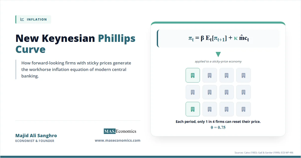
This program produced the modern New Keynesian Phillips Curve, which derives the inflation equation from explicit microfoundations rather than fitting a reduced-form relationship. In its baseline form:
Current inflation depends on expected future inflation \( E_{t}\pi_{t+1} \) discounted by \( \beta \), and on the output gap \( \widetilde{y}_{t} \) scaled by \( \kappa \). The slope \( \kappa \) is derived from price-setting frictions (Calvo or Rotemberg) and preference parameters; the expectations term is genuinely forward-looking under rational expectations.
The New Keynesian framework is supposed to be Lucas-proof in the sense that \( \beta \) and \( \kappa \) are deep parameters that should not change when the policy rule changes. In practice, the empirical record is more mixed. The slope \( \kappa \) estimated on US data has been re-estimated repeatedly across samples, and the estimates have not been stable. Some researchers, including Hazell, Herreño, Nakamura, and Steinsson (2022), have argued that earlier estimates were biased downward by aggregate confounders and that using state-level data produces a steeper and more stable slope. Others argue that even \( \kappa \) is partly a function of indexation, market power, and price-setting institutions, which themselves respond to the inflation environment.
Definition. A deep parameter is one that describes preferences, technology, or fundamental behavior that should not change when policy changes. A reduced-form parameter summarizes an observed relationship that may bundle behavior with the prevailing policy rule. The Lucas critique applies to reduced-form parameters but is supposed to be neutralized by working with deep parameters.
Assumptions and Boundaries
The Lucas critique is built on strong assumptions, and its force depends on how fully they are satisfied. The central assumption is that private agents form expectations rationally, using all available information, including knowledge of the policy rule. If agents are backward-looking, using only past data to form expectations, the coefficients of reduced-form relationships remain stable when policy rules change, at least until the new data eventually alter the adaptive scheme. The critique is then weaker in the short run and may apply with a lag. Behavioural macroeconomics has documented persistent deviations from full rationality, from inertial expectations to diagnostic expectations, that soften the knife-edge of the Lucas argument.
A second assumption is that the policy regime change is understood and believed. A change in the interest-rate rule that the private sector does not perceive, or does not trust to be permanent, will not immediately alter behaviour. The speed and completeness of learning matter. The literature on central bank credibility is in part about how quickly agents internalise a new regime. The Volcker disinflation of 1979–1982 is a classic case. The Federal Reserve’s shift to tight money was initially met with scepticism; wage and price setters continued to expect high inflation for several years, and only after the recession of 1982 did inflation expectations fall sharply. The Lucas critique operated with a credibility lag.
A third boundary is that not all estimated relationships are vulnerable. Relationships that are truly structural, those describing technological constraints, demographic patterns, or laws of nature, are immune. The capital-output ratio in a Cobb-Douglas production function, the Solow residual, or the elasticity of substitution between skilled and unskilled labour are not directly altered by a shift in the monetary policy rule. The critique targets behavioural relationships that embed expectations: consumption functions, investment equations, wage-setting rules, money-demand equations, and any other equation where a decision-maker’s forecast of the future enters explicitly or implicitly.
The critique also requires that the policy rule be systematic. Purely random policy shocks, as opposed to changes in the systematic component, do not alter the reduced-form coefficients in a fundamental way; they are part of the error term and can be handled with standard econometric methods. The problem arises when the systematic part of policy changes, because then the entire correlation structure between instruments and outcomes shifts. This distinction has practical force. A temporary fiscal stimulus in a recession affects the economy but does not change the long-run relationship between taxes and output if the public expects the tax structure to revert. A permanent shift in the marginal tax rate, by contrast, can alter labour supply, saving behaviour, and the measured multiplier on government spending.
Finally, the critique assumes that agents’ decisions embed the entire future path of policy. In realistic settings, decision-making is boundedly rational, and agents use simple heuristics. The formal DSGE models that emerged after Lucas incorporate rational expectations but also recognise that frictions and limited information can dampen the effects the critique describes. The empirical force of the critique is thus a matter of degree, not an all-or-nothing proposition.
Limits of the Lucas Critique
The Lucas critique is one of the most cited results in twentieth-century macroeconomics, but its quantitative bite has been debated. Three counter-arguments deserve attention.
The first is empirical. Christopher Sims, Thomas Sargent, and Lars Hansen all argued at various points that the quantitative magnitude of the Lucas critique, while real, is often smaller than the philosophical force of the argument suggests. In particular, when policy changes are small relative to historical variation, reduced-form models can perform adequately because the regime change is not large enough to move the parameters meaningfully. The critique bites hardest at major regime breaks, not at modest policy adjustments.
The second is that “deep” parameters are not always as deep as the framework claims. Tastes can change, technology evolves, and the structure of labor and product markets shifts over decades in ways that affect even the parameters New Keynesian models treat as primitive. The deep-parameter solution to the Lucas critique is closer to a useful approximation than a guaranteed escape.
The third is closely related. Charles Goodhart’s contemporaneous observation, often summarized as Goodhart’s Law, makes a similar point in a different domain. When a statistical regularity is used as a policy target, the relationship that motivated the target tends to break down. Goodhart’s Law and the Lucas critique are intellectual siblings. Both warn that econometric relationships estimated under one regime cannot be exploited as policy levers in another without changing the underlying behavior that produced the relationship.
Caveat. The Lucas critique applies most strongly to active attempts to exploit a reduced-form relationship for policy gain. It applies less strongly to forecasting under unchanged policy, where reduced-form models can perform well even when their parameters are not deep.
2022 Surge as a Modern Test
The post-pandemic inflation surge has become a useful test case for the Lucas critique in real time. Through the 2010s, the consensus view inside academic and policy circles was that the Phillips Curve had flattened durably. Several papers, including Coibion, Gorodnichenko, and Kamdar’s 2018 survey, argued that the slope of slack was close to zero and that inflation would respond only weakly to labor market tightness. The implied prediction was that a recovery from the pandemic would not generate meaningful inflation, even at very low unemployment.
That prediction failed. Inflation rose sharply in 2021 and 2022, services inflation proved sticky into 2023 and 2024, and the apparent slope of the Phillips Curve steepened during the episode. Rather than concluding the Phillips Curve was wrong, the Lucas reading is that the flat slope of the 2010s was itself a regime artifact. Anchored expectations under a credible inflation target produced a sample in which the slope was hard to identify because inflation barely moved. When shocks were large enough to test the regime (energy and supply chains in 2022), the slope re-emerged. The “Phillips Curve is dead” claim was correct as a description of the previous regime but incorrect as a prediction about future regimes.
The post-Volcker era offered the same lesson in reverse. Models built on the high-inflation 1970s overpredicted the cost of the Volcker disinflation because they did not anticipate the credibility shift. Lucas’s critique applied symmetrically: models calibrated on credibility cannot anticipate non-credibility, and models calibrated on non-credibility cannot anticipate credibility. The same economy, modeled with reduced-form parameters fit to one regime, will mispredict the other.
Implications for Modern Modeling
For practical inflation modeling, three implications follow from the critique that have shaped the discipline since the late 1970s.
The first is the central role of expectations. If the slope of the Phillips Curve depends on how expectations are formed, then modeling expectations explicitly, rather than treating them as a fixed lag of past inflation, becomes essential. This is why the New Keynesian framework places the expectation term \( E_{t}\pi_{t+1} \) front and center. Survey measures of expectations, market-implied measures, and structural estimation methods all became serious research programs in the wake of the critique. As rational expectations theory developed, the question shifted from “what is the trade-off” to “how do agents form their forecasts.”
The second is the importance of policy credibility. If the slope of the trade-off is regime-dependent, then a credible commitment to low and stable inflation can flatten the curve and reduce the output cost of any given inflation deviation. This is the intellectual basis for inflation targeting as a policy framework. The framework’s value is precisely its capacity to anchor the expectation term so that shocks fade quickly rather than becoming embedded in persistence.
The third is methodological humility. Reduced-form inflation forecasts have value, but they should be presented with explicit awareness that the parameters being used reflect the regime that produced them. Modern central bank forecasting suites combine reduced-form models with structural DSGE models, panel-data evidence across regimes, and survey-based expectations precisely to triangulate around the limitations any single approach inherits from the Lucas critique.
Explains
Three concepts that frame the Lucas critique.
Continue with related inflation theory and modeling frameworks.
Explore the MASEconomics BlogConclusion
The Lucas critique reshaped how economists think about inflation modeling by drawing a sharp line between observed empirical regularities and the deep parameters that generate them. The line has been useful even when the implementation has been imperfect. Every major Phillips Curve estimate from the 1960s, 1970s, and 2010s broke down precisely as the critique predicted, because each was built on reduced-form parameters specific to a regime that did not survive contact with the next inflation shock.
What the critique does not deliver is a finished alternative. The deep-parameter program has produced workable models, but the deep parameters themselves have not always behaved as deeply as the framework hoped. Inflation persistence, the Phillips Curve slope, and price-setting frictions all show some sensitivity to the policy environment in which they were estimated. The honest reading is that the Lucas critique narrows the set of empirical claims a careful inflation economist can make, without replacing the need for those claims with a regime-proof alternative. It teaches the discipline a useful habit: always ask which parameters in a model are deep, which are reduced-form, and what the implicit policy regime is when the model was estimated. The 2022 inflation surge made the relevance of that habit visible to anyone who had been comfortable assuming the previous regime would persist.
Frequently Asked Questions
What is the Lucas critique in simple terms?
It is the argument that statistical relationships estimated from historical data cannot be used to predict what will happen if economic policy changes, because the parameters of those relationships are themselves functions of the policy regime that produced the data. When the regime changes, the parameters change, and the forecast is wrong.
Why does the Lucas critique matter for inflation models?
Because the Phillips Curve, the inflation persistence coefficient, and the slope of the inflation-unemployment trade-off are all reduced-form parameters that have shifted with each major change in monetary policy regime. Every major Phillips Curve breakdown since 1970 is consistent with the critique. Treating these parameters as stable produces forecasting failures during regime changes.
What was Lucas’s solution to the critique he raised?
To build macroeconomic models from deep parameters, those describing preferences, technology, and fundamental behavior that should not change when policy changes. The modern New Keynesian framework follows this approach by deriving the inflation equation from explicit microfoundations rather than fitting reduced-form correlations.
Does the Lucas critique mean reduced-form models are useless?
No. Reduced-form models can perform well for forecasting under unchanged policy regimes and for analyzing relationships that are unlikely to be exploited as policy levers. The critique applies most strongly to active attempts to use a reduced-form relationship as the basis for policy choice, where the policy itself changes the relationship being exploited.
How is the Lucas critique related to Goodhart’s Law?
The two are closely related. Goodhart’s Law says that when a statistical regularity is used as a policy target, the relationship that motivated the target tends to break down. The Lucas critique gives a formal econometric statement of why this happens in the context of macroeconomic policy. Both argue that observed relationships are not exploitable in the way naive models suggest, because the behavior generating the relationship responds to the attempt to exploit it.
What does policy invariant mean?
A relationship is policy invariant if its coefficients stay the same when the policy rule changes. The Lucas critique is the claim that reduced-form relationships generally are not, because they mix together genuine structure with the behaviour induced by the prevailing regime. The response is to build models from parameters that plausibly are invariant, such as preferences and technology, and to derive the reduced form from them rather than estimating it directly.
What is the difference between deep and reduced-form parameters?
Deep or structural parameters describe things that do not depend on policy: how much households value present versus future consumption, how readily they substitute between goods, how quickly capital depreciates. Reduced-form parameters are the coefficients of an estimated equation, which are functions of the deep parameters and of the policy rule. Only the deep ones can be carried across a regime change, which is why modern macro models are written in terms of them.
What evidence supports the Lucas critique?
The clearest case is the Phillips curve. The stable trade-off between inflation and unemployment observed in the 1960s broke down in the 1970s once policymakers tried to exploit it, exactly as the argument predicts, because workers began to build the expected inflation into wage demands. Similar breaks appear after the Volcker disinflation, after inflation targeting was adopted in the 1990s, and in money demand equations after financial deregulation.
What are the limits of the Lucas critique?
Three are commonly raised. It is a statement about direction rather than magnitude, and empirically the parameter drift is sometimes small enough to ignore for short horizons. The so-called deep parameters have themselves proved unstable across countries and decades, so the cure is not complete. And a fully structural model buys invariance at the price of strong assumptions that may be wrong in other ways, which is why reduced-form forecasting has never actually been abandoned.
Thanks for reading! If you found this helpful, share it with friends and spread the knowledge. Happy learning with MASEconomics