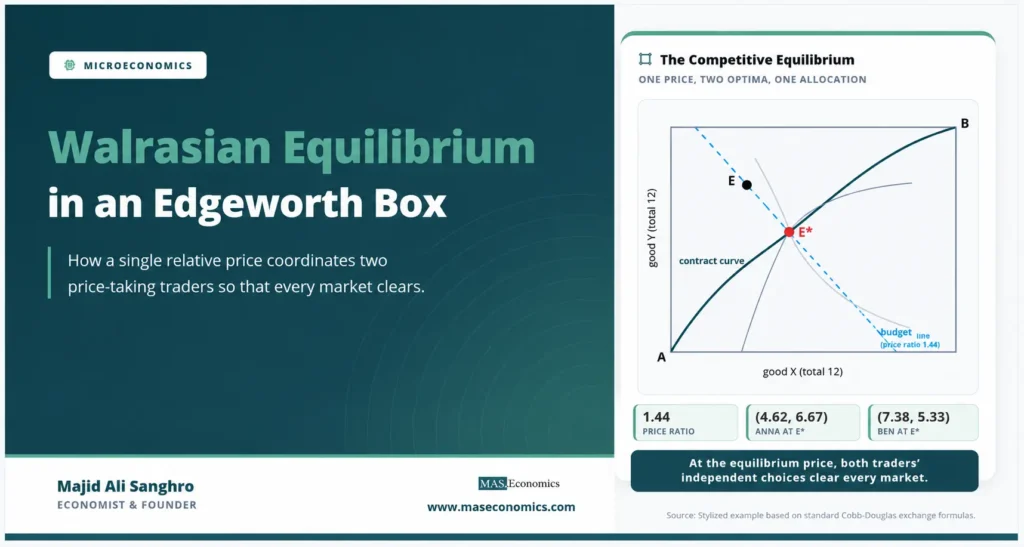
A market has no auctioneer. No central figure calls out a price, listens for excess demand, and adjusts until the books balance. Yet competitive markets behave as if someone did exactly that, and the cleanest place to see why is the two-person, two-good exchange economy drawn inside an Edgeworth box. A Walrasian equilibrium Edgeworth box shows the moment a single relative price does all the coordinating: each trader, looking only at that price and their own holdings, chooses a bundle, and at the right price those independent choices fit together so that every market clears. The budget line that delivers this is the heart of the diagram, and once it is read the abstract idea of a price-taking equilibrium becomes concrete.
The Walrasian, or competitive, equilibrium is named for Léon Walras, who in the 1870s framed the economy as a system of markets that clear simultaneously through prices. In a full economy, that system has thousands of equations. In the box it collapses to one relative price and two traders, which is why the box remains the standard teaching device for the concept. The equilibrium is built step by step: the budget line, its passage through the endowment, each trader’s optimum, and the compatibility of the two optima. The conceptual groundwork is laid in the Edgeworth box and the wider system in general equilibrium analysis.
Box, Endowment, and Price
Take two traders, Anna and Ben, and two goods, X and Y, in fixed total supply. In this example, the economy holds 12 units of each good. Anna’s bundle is read from the bottom-left origin and Ben’s from the top-right origin, so any point in the box is a complete division of the totals. The traders begin at an endowment, the allocation they hold before trade. Here Anna starts with 3 units of X and 9 of Y, written A = (3, 9), and Ben holds the remainder, B = (9, 3). Anna is rich in Y and short of X; Ben is the mirror image.
Now introduce a single relative price. Because only relative prices matter in exchange, fix the price of Y at 1 and let the price of X be \( p \). Each trader values their endowment at these prices to get a money income, then spends that income on the bundle they most prefer. The crucial geometric object is the budget line: the set of bundles a trader can afford given the price and the value of their endowment. In the box, one budget line serves both traders, because a trade that takes goods from one hands them to the other at the same prices.
Budget Line Pivot Through Endowment
The budget line always passes through the endowment point, and the reason is simple. Whatever the price, a trader can always choose not to trade at all and simply consume what they started with. The endowment is therefore affordable at every price, so it lies on every budget line. Changing the price does not shift the line sideways; it pivots the line around the fixed endowment point. The slope of the budget line is the negative of the relative price, \( -p \), since giving up one unit of X frees enough income to buy \( p \) units of Y.
Budget Line
This pivoting is the engine of the whole diagram. A steep budget line means X is expensive relative to Y; a flat one means X is cheap. As the price changes, the line swings through the endowment, and each trader slides to a different preferred bundle along it. The equilibrium price is the particular slope at which the two traders’ preferred bundles describe the same allocation, the point where what Anna wants to buy is exactly what Ben wants to sell.
Each Trader’s Optimal Choice
Facing the budget line, a trader picks the affordable bundle on the highest reachable indifference curve. Geometrically, that is the point where an indifference curve is tangent to the budget line. At a tangency the slope of the indifference curve equals the slope of the budget line, which means the trader’s marginal rate of substitution equals the relative price.
Consumer Optimum
Suppose Anna has equal-weight Cobb-Douglas preferences, so she spends half her income on each good, while Ben weights X more heavily and spends two-thirds of his income on X. These preference differences are what give the example its bite: the two traders respond differently to the same price, and finding the price that reconciles them is the work of the equilibrium. As the price varies, each trader’s optimum traces out an offer curve, the locus of preferred bundles across all prices. The Walrasian equilibrium is where the two offer curves intersect, away from the endowment.
Solving for Equilibrium Price
The equilibrium is the price at which both markets clear. With the price of Y normalized to 1, Anna’s income is the value of her endowment, \( M_A = 3p + 9 \), and Ben’s is \( M_B = 9p + 3 \). Anna spends half her income on X, so her demand for X is \( 0.5 M_A / p \). Ben spends two-thirds on X, so his demand is \( (2/3) M_B / p \). Market clearing for X requires the two demands to sum to the total supply of 12.
Market Clearing for X:
Multiplying through by \( p \) and collecting terms gives \( 1.5p + 4.5 + 6p + 2 = 12p \), which simplifies to \( 7.5p + 6.5 = 12p \), so \( 4.5p = 6.5 \) and \( p = 13/9 \approx 1.44 \). The relative price of X settles above 1, reflecting that X is the good both traders lean toward, Ben especially, relative to the supply. By Walras’ law, once the market for X clears, the market for Y clears automatically, so this single equation pins down the equilibrium.
The equilibrium price is not chosen by anyone. It is the value that makes independent, self-interested choices mutually consistent. Above it, more X is demanded than exists; below it, less. Only at the equilibrium price do the two traders’ plans fit together exactly.
Equilibrium Allocation
Substituting \( p = 13/9 \) back into the demands gives the final bundles. Anna’s income is \( M_A = 3(13/9) + 9 \approx 13.33 \), so she demands about 4.62 units of X and 6.67 units of Y. Ben’s income is \( M_B = 9(13/9) + 3 = 16 \), so he demands about 7.38 units of X and 5.33 units of Y. The two demands for X sum to 12 and the two for Y sum to 12, so both markets clear exactly.
| Trader | Endowment (X, Y) | Equilibrium (X, Y) | Net trade | MRS at equilibrium |
|---|---|---|---|---|
| Anna | (3, 9) | (4.62, 6.67) | +1.62 X, −2.33 Y | 1.44 |
| Ben | (9, 3) | (7.38, 5.33) | −1.62 X, +2.33 Y | 1.44 |
| Totals | (12, 12) | (12, 12) | Balanced | Equal to price |
|
Source: Stylized example based on standard Cobb-Douglas exchange formulas.

|
||||
Two features confirm the result. The net trades are equal and opposite, as conservation of goods requires: Anna buys the 1.62 units of X that Ben sells, and Ben buys the 2.33 units of Y that Anna sells. And both traders’ marginal rates of substitution equal the common price of 1.44, which is the tangency condition for efficiency. The equilibrium therefore lies on the contract curve, the set of efficient allocations explored in our companion piece on the contract curve and Pareto efficient allocations.
Equilibrium in the Diagram
The whole solution sits in one figure. The budget line pivots through the endowment with slope equal to the negative equilibrium price. Each trader’s highest reachable indifference curve is tangent to that line at the same point, the equilibrium allocation. Because both tangencies occur at one point, the two indifference curves are tangent to each other there as well, which places the equilibrium on the contract curve.
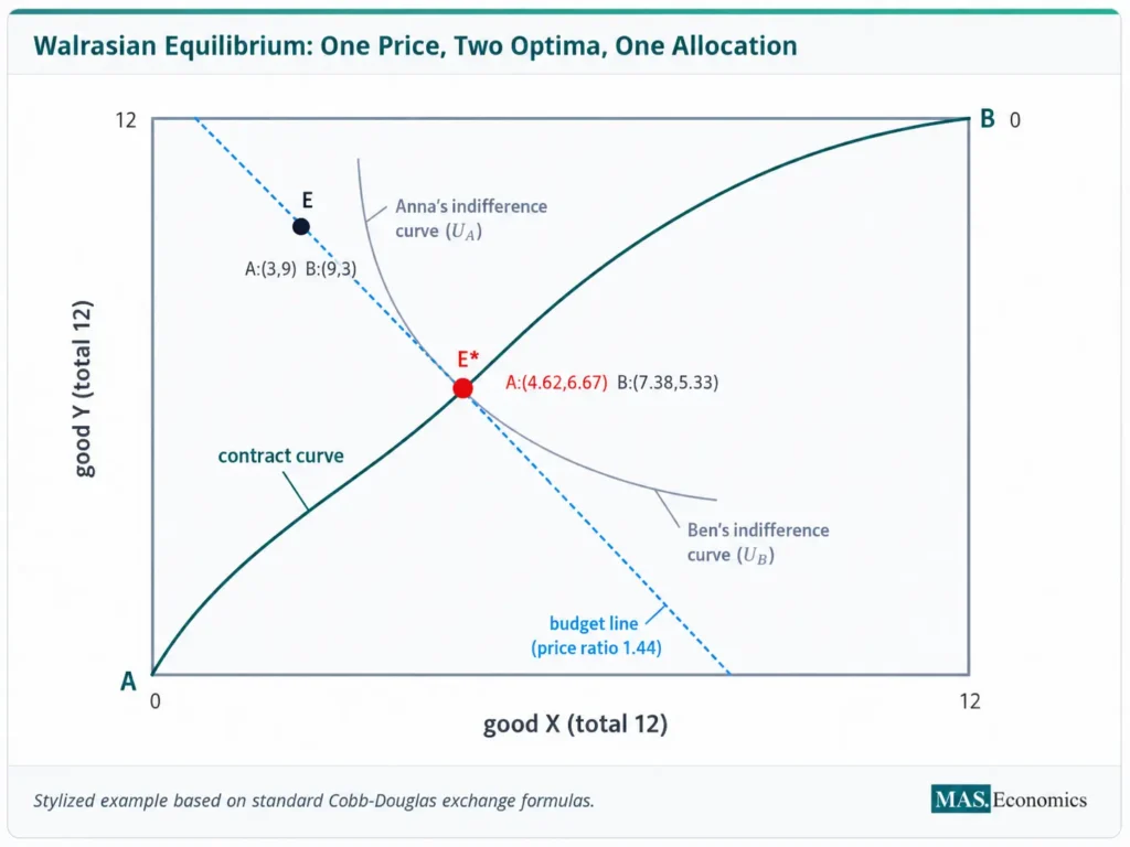
The endowment E lies off the contract curve, so it is inefficient and gains from trade remain. The dashed blue budget line passes through E, as it must, and through E* at slope 1.44. At E* one of Anna’s indifference curves and one of Ben’s are both tangent to the budget line, so the two curves touch each other there. That is the Walrasian equilibrium: a single price, two independently optimizing traders, and one allocation on which their plans agree.
Existence, Walras’ Law, and Welfare
Three properties make the construction more than a single solved example. The first is Walras’ law: the combined value of all excess demands is zero at any price, because each trader’s spending is constrained by the value of their endowment. This is why clearing one market guarantees the other clears, and why a two-good economy needs only one relative price. The second is existence. Under standard assumptions, convex preferences and continuous demands, at least one equilibrium price exists, so the diagram is not a lucky special case. The third connects the construction to welfare.
Because every trader sets their marginal rate of substitution equal to the same price, all traders’ marginal rates of substitution are equal to one another at the equilibrium. That is precisely the condition for Pareto efficiency, so a competitive equilibrium is efficient. This is the First Welfare Theorem, and the box is its simplest proof. The Second Welfare Theorem runs the other way: any efficient allocation on the contract curve can be reached as a competitive equilibrium by first choosing the right endowment. Together, these results, developed in welfare economics and Pareto efficiency, explain why economists treat competitive prices as a decentralized way of reaching efficient outcomes. The same machinery, solved with different numbers, appears in our worked Edgeworth box examples.
Explains
Three ideas behind the competitive equilibrium
Explore related explainers on prices, exchange, and efficiency.
Explore the MASEconomics BlogConclusion
The Walrasian equilibrium Edgeworth box distills the idea of a competitive market to its essentials: a single relative price, a budget line pivoting through the endowment, and two price-taking traders who each choose a tangency on that line. The equilibrium is the price at which those two independent choices describe one allocation, so every market clears without any coordinator setting quantities. In the worked example, an endowment of A = (3, 9) and B = (9, 3) with different Cobb-Douglas weights produced an equilibrium price ratio of about 1.44 and a final allocation of A = (4.62, 6.67) and B = (7.38, 5.33).
The diagram does more than locate that allocation. It shows why the equilibrium must be efficient, since equal marginal rates of substitution across traders place the outcome on the contract curve, and it shows why Walras’ law lets one price clear both markets. The box is small, but the lesson scales: in a full economy, the same logic, prices reconciling decentralized choices, is what a competitive market does, and the First Welfare Theorem is the formal statement that, under its assumptions, the result is efficient.
Frequently Asked Questions
What is a Walrasian equilibrium in an Edgeworth box?
It is a relative price at which two price-taking traders, each choosing their most preferred affordable bundle, end up with plans that fit together so both markets clear. In the box it appears as a budget line through the endowment whose slope is the equilibrium price, tangent to one indifference curve of each trader at the same point. That common point is the competitive equilibrium allocation.
Why does the budget line pass through the endowment?
Because a trader can always choose not to trade and simply consume their endowment, which means the endowment is affordable at any price. Since it is always affordable, it lies on every budget line. Changing the price does not move the line sideways; it pivots the line around the fixed endowment point, changing its slope.
How do you find the equilibrium price?
Set one good as the numeraire with price 1, value each trader’s endowment to get income, and write each trader’s demand as a function of the price. Impose market clearing for one good, meaning total demand equals total supply, and solve for the price. By Walras’ law the other market then clears automatically, so a single equation determines the relative price.
Is a Walrasian equilibrium always efficient?
Under standard assumptions, yes. At a competitive equilibrium every trader sets their marginal rate of substitution equal to the same price ratio, so all traders’ rates are equal to one another. That is the tangency condition for Pareto efficiency, which places the equilibrium on the contract curve. This result is the First Welfare Theorem.
What is the difference between the contract curve and the Walrasian equilibrium?
The contract curve is the whole set of efficient allocations, defined by preferences and total resources. The Walrasian equilibrium is the single efficient allocation that competitive prices select from a given endowment. The equilibrium always lies on the contract curve, but which point it lands on depends on the endowment, since that determines each trader’s income.
Thanks for reading! If you found this helpful, share it with friends and spread the knowledge. Happy learning with MASEconomics