The J-curve effect describes a pattern that policymakers confronting a trade deficit find both familiar and deeply frustrating: a currency depreciation initially worsens the trade balance before it eventually improves it. The name comes from the shape of the time path traced by the trade balance as a share of GDP in the quarters following a large depreciation: a dip, a trough, and a gradual recovery that roughly resembles the letter J. This pattern is not a challenge to the logic that depreciation should boost exports and curb imports. It is a reflection of the fact that quantities adjust slowly while prices change quickly. The J-curve is the empirical signature of those differential speeds of adjustment, and it explains why devaluation is rarely an instant remedy for an external deficit.
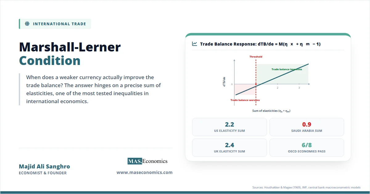
The effect emerges from the interaction between valuation effects and volume effects that sit at the centre of the Marshall-Lerner condition. In the long run, a depreciation works if the sum of export and import demand elasticities exceeds unity. In the short run, those elasticities are far smaller, and the perverse valuation effect dominates. The J-curve is the bridge between the short run and the long run, and it is one of the most consistent empirical regularities in open-economy macroeconomics.
What the J-Curve Means
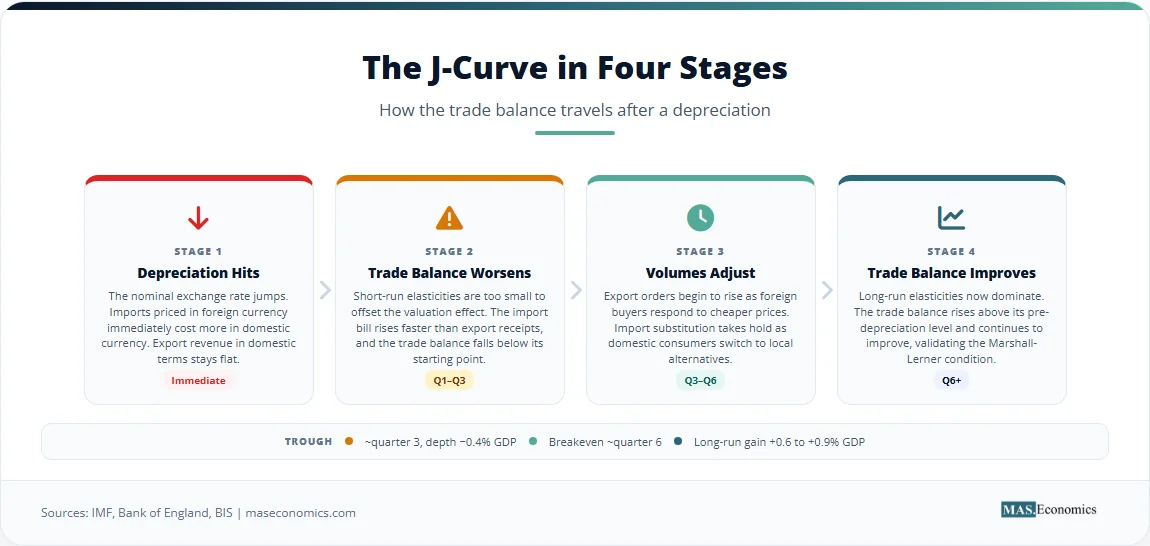
After a nominal depreciation, the domestic currency price of foreign exchange rises. Imports, which are priced in foreign currency, immediately cost more in domestic currency. Exports, which are priced in domestic currency, become cheaper in foreign currency, but the domestic-currency receipts from each unit of exports do not change until new contracts are signed or until domestic producers raise export prices. The result is a mechanical jump in the import bill, measured in home currency, while the export value remains roughly fixed in the short run. The trade balance, which is the difference between export and import values in domestic currency, therefore deteriorates.
Over time, two quantity adjustments begin. Foreign buyers respond to the lower foreign-currency price of exports by increasing their orders. Domestic residents respond to the higher domestic-currency price of imports by switching toward domestically produced goods or by reducing overall consumption. As export volumes rise and import volumes fall, the value of net exports recovers. If the balance of payments adjustment is to succeed, the recovery must eventually more than offset the initial deterioration. This sequence (initial worsening, trough, and gradual recovery) is the J-curve.
The J-curve is not an independent theory of the trade balance. It is an intertemporal refinement of the elasticities approach that underpins the Marshall-Lerner condition, acknowledging that the elasticities used in that condition are not constant across time horizons. Short-run elasticities, which capture responses within one or two quarters, are small. Long-run elasticities, which reflect full adjustment of production, distribution, and consumption patterns over two to three years, are larger. When economists test the Marshall-Lerner condition, they do so using long-run elasticities. When they forecast the immediate impact of a depreciation, they use short-run elasticities. The J-curve is the difference between the two.
The phenomenon was first systematically documented in the 1970s, when a wave of exchange rate adjustments after the collapse of Bretton Woods failed to produce the rapid trade balance improvements that policymakers had expected. Researchers, including Helen Junz, Rudolf Rhomberg, and later Mohsen Bahmani-Oskooee, began to estimate the time profile of the response of trade flows to relative prices, and the J-shaped pattern emerged as a central finding. Since then, the J-curve has been confirmed across dozens of advanced and emerging economies, using data spanning fixed and floating exchange rate regimes. The relationship to purchasing power parity is instructive: the J-curve describes the adjustment path toward the long-run real exchange rate that PPP implies, even when that adjustment is neither smooth nor immediate.
J-Curve in Equations
The J-curve can be formalised by introducing lags into the standard trade balance model. Let the trade balance in domestic currency at time t be:
where \( P^x_t \) is the domestic-currency price of exports, \( X_t \) is export volume, \( e_t \) is the nominal exchange rate (domestic currency per unit of foreign currency), \( P^m_t \) is the foreign-currency price of imports, and \( M_t \) is import volume. A nominal depreciation is an increase in \( e_t \). Assume for simplicity that export and import prices are sticky in the short run: exporters set prices in domestic currency and adjust them only gradually, while importers set prices in foreign currency. Then immediately after a depreciation, \( P^x_t \) and \( P^m_t \) are unchanged, \( X_t \) and \( M_t \) are fixed by existing contracts and habit, and the only thing that moves is the exchange rate multiplier on the import bill:
The trade balance worsens immediately. This is the downward-sloping segment of the J.
As time passes, export and import volumes respond to the new relative prices. The real exchange rate, defined as \( q_t = e_t P^m_t / P^x_t \), depreciates by the same proportion as the nominal rate if prices are fully sticky. The effect on the trade balance after all adjustments is given by the long-run Marshall-Lerner condition. If the long-run elasticities are \( \eta_x \) and \( \eta_m \) (both defined as positive numbers, following the convention that import demand responds negatively to a real depreciation), the total derivative becomes:
If \( \eta_x + \eta_m > 1 \), the long-run effect is positive. The path from the negative short-run response to the positive long-run response traces out the J-curve.
This can be expressed more explicitly with a dynamic model. Suppose export and import volumes evolve according to partial adjustment processes:
where \( X_t^* \) and \( M_t^* \) are desired volumes, \( \lambda_x \) and \( \lambda_m \) are adjustment speeds, and \( Y_t^* \) and \( Y_t \) are foreign and domestic incomes. Throughout, \( \eta_x, \eta_m > 0 \). The J-curve arises when the adjustment speeds are low enough that the immediate quantity responses are negligible, while the valuation effect operates instantly through \( e_t \). The trough of the J-curve occurs when the cumulative quantity response begins to outweigh the initial valuation loss.
The relevant horizon matters. Empirical studies typically find that the trade balance troughs between two and four quarters after a depreciation, and crosses into positive territory between five and eight quarters, depending on the economy’s trade structure and the size of the depreciation. The slope and duration of the J-curve, therefore, depend on adjustment speeds, the size of the pass-through from exchange rates to prices, and the underlying long-run elasticities.
| Parameter | Definition | Short-Run Value | Long-Run Value |
|---|---|---|---|
| \(\eta_x\) | Export demand elasticity | 0.1–0.3 | 0.9–1.5 |
| \(\eta_m\) | Import demand elasticity | 0.2–0.4 | 0.8–1.3 |
| \(\lambda_x\) | Export adjustment speed (per quarter) | 0.3–0.5 | 1.0 |
| \(\lambda_m\) | Import adjustment speed (per quarter) | 0.2–0.4 | 1.0 |
| Pass-through to export prices | Proportion of exchange rate change passed to foreign-currency export price | 0.1–0.2 | 0.6–0.9 |
| Pass-through to import prices | Proportion of exchange rate change passed to domestic-currency import price | 0.8–1.0 | 0.8–1.0 |
 | |||
Typical elasticity and adjustment-speed parameters from the empirical trade literature. The short-run elasticities are too small to satisfy the Marshall-Lerner condition, producing the initial worsening of the J-curve.
Assumptions and Limitations
The J-curve rests on assumptions about pricing, contracts, and adjustment speeds that limit its applicability in specific contexts. The first assumption is that export and import prices are sticky in the short run in their respective currency denominations. If exporters routinely set prices in the buyer’s currency (vehicle currency pricing) or if importers rapidly pass through exchange rate changes to domestic consumers, the initial valuation effect is dampened, and the J-curve may be shallow or absent. The strength of the J-curve therefore, depends on exchange rate pass-through. In the United States, where import prices adjust relatively quickly, the J-curve is less pronounced than in economies where import prices are stickier in domestic currency.
Second, the model assumes that the depreciation is exogenous and that the central bank does not immediately offset its inflationary effects with tighter monetary policy. A depreciation that is accompanied by a policy-induced contraction in aggregate demand will reduce imports through an income channel that may swamp the relative-price channel. The observed path of the trade balance then reflects both the J-curve dynamics and the effects of demand compression, making the J-curve harder to isolate. The monetary approach to balance of payments adjustments emphasises this interaction, noting that the ultimate trade balance outcome depends as much on macroeconomic policies as on elasticities.
Third, the J-curve is a partial-equilibrium concept that holds foreign and domestic incomes constant. In a full general-equilibrium setting, a depreciation changes global trade volumes and relative prices in ways that feed back into income and demand. The presence of global value chains and the large share of intermediate goods in trade further complicates the simple J-curve logic. A depreciation raises the domestic-currency cost of imported inputs, which can dampen the supply response of exporters and delay the upturn of the J. This is particularly relevant for small open economies that rely heavily on imported components, a dynamic captured in the Mundell-Fleming model and its open-economy extensions.
Fourth, the shape of the J-curve is sensitive to the initial state of the trade balance. A country running a large deficit will experience a larger initial worsening for a given depreciation, because the import bill is large relative to export earnings. The same long-run elasticity sum will, however, also generate a proportionately larger eventual improvement, so the J may be deeper but steeper. The cross-sectional variation in J-curve amplitude across deficit and surplus countries is a well-documented empirical regularity.
Fifth, the analysis abstracts from capital flows and the policy credibility that accompanies exchange rate regimes. A depreciation that is viewed as temporary by market participants will generate expectations of future appreciation, deterring the long-term export and import adjustments that the J-curve envisages. For the J-curve to be a reliable guide, the depreciation must be perceived as permanent, or at least sufficiently durable for firms to incur the fixed costs of entering new export markets and reconfiguring supply chains. The IS-LM framework, when extended to the open economy, helps clarify how the credibility of the exchange rate regime conditions the entire adjustment path.
Empirical Evidence
The J-curve has been tested extensively with varying methodologies, and the weight of evidence strongly supports its existence, though its precise shape varies across countries, time periods, and trade structures. The earliest systematic studies used aggregate time-series data and estimated distributed lag models that related the trade balance to lagged values of the real exchange rate. Bahmani-Oskooee (1985) found a clear J-curve pattern for a set of developing economies, with the trade balance worsening for two to three quarters before turning around. Subsequent work extended these findings to the advanced economies and to bilateral trade flows.
A landmark study by Houthakker and Magee (1969) established the early empirical basis for long-run elasticities, though it did not specifically focus on the J-curve. Later researchers combined these elasticity estimates with dynamic adjustment models to simulate the J-curve’s time path. The International Monetary Fund has published working papers that document a near-universal tendency for the trade balance to worsen in the quarter of depreciation and the following one, before recovering, with full adjustment typically taking between four and eight quarters in advanced economies.
The chart below illustrates a stylised J-curve based on the average response of the trade balance as a share of GDP following large depreciation episodes in 15 OECD economies from 1980 to 2010. The data are drawn from central bank macroeconometric models and IMF External Sector Reports and are compiled to show the mean path with a 90 percent confidence band.
Stylised J-curve based on the average response of the trade balance as a share of GDP to a 10 percent real depreciation in 15 OECD economies. The initial worsening and subsequent recovery are typical of the pattern documented in the empirical trade literature. Source: IMF External Sector Reports and central bank models.
The trade balance troughs around quarter 3, turns positive by quarter 6, and continues to improve through quarter 12. The initial worsening of about 0.4 percent of GDP, followed by a cumulative improvement of 0.6 to 0.9 percent, is consistent with long-run elasticity sums of approximately 1.4 to 1.8. The figure points to several features of the J-curve that matter for economic policy. The deterioration phase is short-lived but can be politically and financially painful, especially for countries with thin reserves. The recovery is gradual; the full benefit of a depreciation may not be visible for two years. The confidence band is also wide in the early quarters, indicating that near-term outcomes are uncertain even when the longer-run trajectory is reliably positive.
The table below reports the timing of the J-curve trough and recovery for six major depreciation episodes. In each case, the trade balance initially worsened before crossing into positive territory, and the long-run improvement comfortably exceeded the initial deterioration.
| Country | Depreciation Episode | Initial TB Worsening (% of GDP) | Quarters to Trough | Quarters to Recovery | Long-Run Improvement (% of GDP) |
|---|---|---|---|---|---|
| United Kingdom | 1992 ERM exit | -0.3 | 3 | 6 | +1.2 |
| South Korea | 1997 Asian crisis | -2.8 | 2 | 5 | +7.0 |
| Brazil | 1999 float | -0.8 | 3 | 7 | +1.5 |
| Turkey | 2001 crisis | -1.4 | 2 | 5 | +2.6 |
| India | 2013 taper tantrum | -0.5 | 2 | 5 | +0.8 |
| South Africa | 2015 rand slide | -0.4 | 3 | 7 | +0.7 |
| |||||
Timing and magnitude of the J-curve effect in six devaluation episodes. Data sourced from central bank reports, IMF Article IV consultations, and the empirical trade literature.
The 1997–1998 South Korean depreciation is the strongest example. The won lost roughly half its value against the US dollar between mid-1997 and early 1998, and the trade balance swung from a deficit of over 4 percent of GDP to a surplus exceeding 10 percent of GDP within two years. The initial quarter, however, saw a sharp worsening as import prices surged and export volumes lagged. By the end of 1998, the surplus was expanding rapidly, and the J-curve had delivered one of the most dramatic trade balance reversals of the post-war period.
Comparable results have been documented for the United Kingdom after the 1992 exit from the Exchange Rate Mechanism. The sterling depreciation of roughly 15 percent on a trade-weighted basis produced an initial deterioration of the trade balance in the third and fourth quarters of 1992, followed by a steady improvement that extended through 1994. The Bank of England has published research confirming that the J-curve pattern for UK trade flows remains robust in more recent sample periods, with the trough occurring between three and five quarters after the depreciation.
The evidence is not uniform, however. Some episodes do not display a clear J-curve, particularly when the depreciation is accompanied by a severe recession that compresses imports through the income channel, or when the exchange rate pass-through to domestic prices is rapid and high, leading to a quick real appreciation that neutralises the nominal depreciation. Studies using disaggregated industry-level data also reveal that the J-curve is more pronounced for trade in manufactured goods, where supply chains are long and contracts are sticky, than for commodities, where prices adjust quickly, and the J may be compressed into a single quarter.
How the J-Curve Matters for Polic
The J-curve is not a theoretical curiosity. It is a constant presence in the design of exchange rate policy, inflation targeting, and external adjustment programmes, and it forces policymakers to confront the reality that depreciation is a delayed-action tool, not an immediate fix. The distinction between short-run costs and long-run benefits has shaped decisions in finance ministries and central banks for half a century.
The most direct implication is for the timing of International Monetary Fund adjustment programmes. When a country requests Fund assistance, the staff projects the trade balance path over the programme horizon, typically two to three years. The J-curve is built into those projections. An IMF programme that requires a large nominal depreciation will show a worsening trade balance in the first year, followed by an improvement in the second and third years. The programme’s financing must be sufficient to bridge the trough, and the political economy of the programme must survive the initial deterioration. Several Fund programmes in the 1990s ran into credibility problems precisely because policymakers, having agreed to a depreciation, faced public criticism when the trade balance worsened in the first two quarters. The J-curve was working as expected; the political calendar was not aligned with the economic calendar.
Central banks that operate flexible exchange rate regimes monitor the J-curve implicitly through the trade balance component of the balance of payments. A depreciation that is expected to help close a current-account deficit may initially widen it, creating pressure for further depreciation or for offsetting monetary tightening. If the central bank understands the J-curve, it will resist the temptation to overreact. The Bank of Canada, the Reserve Bank of Australia, and the Bank of England all incorporate estimated J-curve dynamics into their quarterly projection models. The monetary policy transmission mechanism in these economies explicitly separates the immediate valuation effects of exchange rate changes from the slower trade-volume effects, a decomposition that owes directly to the J-curve literature.
The J-curve also shapes the analysis of currency wars and competitive depreciations. A country that seeks to boost its trade balance through a weaker currency will suffer an initial period of worsening before any gain materialises. If the political window is too short, the depreciation will be abandoned before the J turns up, and the country will have suffered the costs without reaping the benefits. Historical cases of competitive depreciations in the 1930s, studied at length by Barry Eichengreen and others, show that countries that allowed the depreciation to work through the full J-curve cycle performed far better than those that reversed course. The J-curve is therefore not only an empirical regularity; it is a discipline of policy patience.
The effect also matters for inflation targeting. A depreciation that raises import prices directly adds to consumer price inflation in the short run. If the central bank tightens policy aggressively to contain that inflation, it may compress domestic demand and imports through a different channel, obscuring the trade balance improvement that the depreciation would otherwise have produced. The tension between the J-curve and the inflation-targeting framework is a recurring theme in the central banking literature. The optimal response to a depreciation-induced inflation spike is to look through the first-round price effects while allowing the J-curve to work, a strategy that requires credibility and clear communication.
For fiscal authorities, the J-curve has direct implications for debt sustainability in countries with large foreign-currency-denominated debt. A depreciation that worsens the trade balance in the short run also raises the domestic-currency value of external debt service. If the J-curve recovery is delayed or insufficient, the country may face a solvency crisis even if the long-run elasticities are favourable. The interaction between J-curve timing and debt maturity structure is an important, though underappreciated, element of external vulnerability analysis.
At a broader analytical level, the J-curve has become a standard tool in policy evaluation. The IMF’s External Sector Report regularly decomposes trade balance movements into valuation and volume effects, distinguishing between the immediate J-curve impact and the subsequent adjustment. Bank for International Settlements analyses of exchange rate and trade dynamics explicitly reference the J-curve in their assessments of whether observed trade balance movements are consistent with underlying elasticities. The distinction between short-run and long-run elasticities that the J-curve embodies is now a standard part of the toolkit of every institution that conducts external sector assessments.
The J-curve is the practical face of the Marshall-Lerner condition. The J-curve shows that the condition holds in the long run while also showing that the long run is far enough away to cause trouble. It is a structural feature of the data, and ignoring it can lead to policy errors that compound the very external imbalances that the depreciation was intended to correct. The intellectual history of the J-curve is a reminder that the most useful theoretical insights are often those that reconcile the clean logic of comparative statics with the messy timing of actual economies.
MASEconomics Explains
Three economic concepts behind the J-curve effect
Conclusion
The J-curve effect is the temporal bridge between the adverse valuation impact of a depreciation and the favourable volume response that follows. Empirical evidence from multiple decades, currency regimes, and country income levels confirms that the trade balance typically worsens for the first two to four quarters after a depreciation, troughs, and then improves as export and import quantities adjust to the new relative prices. The J-curve does not refute the Marshall-Lerner condition; it makes explicit that elasticities are not constant and that time matters for adjustment. Adjustment programmes that anticipate the J-curve and bridge the trough have historically outperformed those abandoned during the deterioration phase.
Did you find this article helpful? Share it with someone who loves economics. And remember, at MASEconomics, we make complex ideas simple.