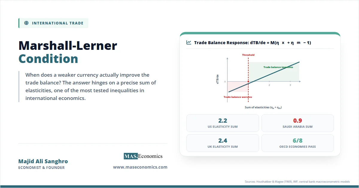
The Marshall-Lerner condition answers a question that has confronted policymakers from the Bretton Woods era to the present: will a currency depreciation improve the trade balance, or will it worsen it? The condition, formalised by Abba Lerner in 1944 but rooted in Alfred Marshall’s earlier work on elasticities, states that a depreciation improves the trade balance if the sum of the price elasticities of demand for exports and imports exceeds one in absolute value. When a country’s currency weakens, exports become cheaper for foreign buyers and imports become more expensive for domestic residents. Whether the trade balance improves hinges on whether the quantity responses are large enough to outweigh the adverse terms-of-trade effect: each unit of exports now earns less foreign currency. The Marshall-Lerner condition gives the precise threshold at which the quantity effects dominate.
The condition sits at the centre of open-economy macroeconomics and remains a standard reference point in the analysis of balance of payments adjustment. It appears in every undergraduate international trade syllabus and underpins the policy advice that devaluation can work, but only under specific elasticity conditions. Its simplicity masks a deep structural logic, and its empirical track record has been scrutinised for more than seven decades.
What the Marshall-Lerner Condition Means
Consider a country that imports and exports goods. The trade balance in domestic currency is the difference between the value of exports and the value of imports, measured in the home currency. If the domestic currency depreciates, the price of foreign currency rises, so each unit of exports now earns more home-currency units while each unit of imports costs more. But consumers and firms in both countries respond to price changes: the quantity of exports demanded by the rest of the world rises because the goods are cheaper in foreign-currency terms, and the quantity of imports demanded by domestic residents falls because foreign goods are now more expensive in home-currency terms.
Two effects pull in opposite directions. The price effect of a depreciation is perverse: a higher exchange rate makes the import bill rise for any given quantity of imports, worsening the trade balance. The quantity effects work to improve it: exports expand and imports contract. The Marshall-Lerner condition is the requirement that the sum of the two quantity elasticities be large enough to overcome the perverse price effect and generate a net improvement. This insight connects directly to the broader monetary approach to balance of payments adjustments, which views exchange rate changes as one of several mechanisms for restoring external equilibrium.
The condition is formally derived under the assumption that the economy starts from a position of balanced trade, so that exports and imports are equal in value. If the initial trade balance is not zero, the condition takes a slightly more general form, but the balanced-trade version is the benchmark that entered the policy debate after the Second World War. It was invoked repeatedly during the fixed-but-adjustable exchange rate regime of Bretton Woods and later during the managed floats of the 1970s and 1980s, as countries sought to understand whether the elasticities of their trade flows were large enough for depreciation to be an effective adjustment tool.
The Marshall-Lerner Condition in Equations
Start with a simple model of the trade balance, TB, expressed in domestic currency. Exports, X, depend on the real exchange rate, e, and on foreign income, Y*. Imports, M, depend on the real exchange rate and on domestic income, Y. The real exchange rate is defined as the relative price of foreign goods in terms of domestic goods, so a rise in e denotes a real depreciation. For analytical purposes, write the trade balance as:
Here, e multiplies M because imports are originally priced in foreign currency, and multiplying by e converts them to domestic-currency terms. The expression captures the dual role of e: it enters positively through the export function, since a depreciation makes home goods cheaper abroad and raises X, and it enters negatively through the valuation of the import bill, since a higher e raises the domestic-currency cost of each imported unit.
Differentiate TB with respect to e, holding incomes constant, and assume that the initial trade balance is zero so that X = e M. Denote the price elasticity of export demand as \(\eta_x = \frac{\partial X}{\partial e} \cdot \frac{e}{X}\), and the price elasticity of import demand as \(\eta_m = -\frac{\partial M}{\partial e} \cdot \frac{e}{M}\), where the minus sign makes \(\eta_m\) positive under normal downward-sloping demand. Both elasticities are defined as positive numbers. After some manipulation, the total derivative is:
The sign of dTB/de is therefore determined by the sign of (\(\eta_x + \eta_m – 1\)). A depreciation improves the trade balance if and only if:
This is the Marshall-Lerner condition in its simplest, balanced-trade form. If the sum of the export and import elasticities exactly equals one, the depreciation leaves the trade balance unchanged. If the sum is less than one, the depreciation worsens it, because the adverse valuation effect on the import bill outweighs the volume response.
The derivation highlights three critical assumptions. First, trade is initially balanced; if a country is running a deficit, the condition must be suitably modified, and a depreciation is more likely to work because the initial value of imports exceeds exports, making the perverse price effect relatively smaller. Second, supply elasticities are infinite, so producers can meet any increase in demand without rising marginal cost. Third, there are no cross-price effects between traded and non-traded goods and no capital flows that might offset current-account movements. These assumptions are relaxed in richer models, including those that underpin the Heckscher-Ohlin model with its factor-endowment determination of trade patterns, but the benchmark version remains the pedagogical and analytical standard.
The variables used in the derivation are summarised in the table below.
| Symbol | Definition | Sign Convention |
|---|---|---|
| TB | Trade balance in domestic currency | Surplus positive |
| X | Export volume | Quantity demanded by foreigners |
| M | Import volume | Quantity demanded by domestic residents |
| e | Nominal or real exchange rate (domestic currency per unit of foreign) | Rise = depreciation |
| Y* | Foreign income | Exogenous |
| Y | Domestic income | Exogenous |
| \(\eta_x\) | Price elasticity of export demand (absolute value) | Positive |
| \(\eta_m\) | Price elasticity of import demand (absolute value) | Positive |
 | ||
Variable definitions for the basic Marshall-Lerner framework. Both elasticities are expressed as positive numbers after applying absolute value notation.
The condition generalises straightforwardly. If the initial trade balance is not zero, the critical value becomes \(\eta_x + (X/eM) \eta_m > 1\), so that a country running a deficit can satisfy the condition with a lower sum of elasticities. If supply is less than perfectly elastic, the required sum of elasticities is higher than one, because a depreciation drives up domestic costs and erodes the competitiveness gain. The benchmark nonetheless captures the central insight: elasticities matter, and there is a precise threshold below which exchange rate adjustment becomes counterproductive. The relationship to the Stolper-Samuelson theorem is instructive: just as trade liberalisation can create winners and losers within a country, devaluation can have distributional effects that depend on the same elasticity structures.
Key Assumptions and Practical Limitations
The Marshall-Lerner condition, despite its elegance, rests on a set of simplifying assumptions that must be evaluated in each application. The first is the assumption of a perfectly elastic supply. If domestic producers face capacity constraints or rising marginal costs, the export response to a depreciation is dampened, and the critical elasticity sum rises above one. This matters for commodity exporters, where output is slow to adjust, and for economies near full employment.
Second, the condition is derived for a partial-equilibrium framework that holds domestic and foreign income constant. In practice, a depreciation changes domestic and foreign real incomes through expenditure-switching and terms-of-trade effects, and these income changes feed back into trade volumes. General-equilibrium models embed the Marshall-Lerner logic but recognise that income effects can amplify or offset the direct elasticity channel. The Mundell-Fleming model and its modern descendants incorporate the condition as part of a broader adjustment process in which monetary and fiscal policies also shift.
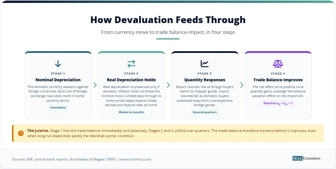
Third, the condition ignores short-run dynamics. Empirical evidence, associated with the J-curve, shows that the trade balance often worsens in the months immediately following a depreciation before improving later. Pre-existing contracts, sticky quantities, and slow consumer recognition of relative price changes delay the quantity responses, while the perverse valuation effect hits immediately. The Marshall-Lerner condition does not contradict this pattern; it specifies the long-run outcome after quantities have fully adjusted. The distinction between short-run and long-run elasticities, and the time path by which the latter are approached, is a major theme in the empirical literature on exchange rates and trade.
Fourth, the condition assumes that the depreciation is real, not merely nominal. If a nominal depreciation is quickly offset by domestic inflation, the real exchange rate does not change, and the quantity responses never materialise. This is why “pass-through” is central: the degree to which exchange rate changes are reflected in import and export prices determines whether the real depreciation required for the Marshall-Lerner condition actually occurs. In economies with high inflation pass-through, nominal devaluations often fail to deliver real depreciation, and the condition is not met even when elasticities are favourable.
Finally, the derivation abstracts from cross-border capital flows. A depreciation that improves the trade balance also generates an incipient surplus on the current account, which must be matched by capital outflows. If these flows affect the exchange rate itself, through portfolio rebalancing, the initial depreciation may be partly reversed. The condition is best viewed as a necessary but not sufficient element of a sustainable balance of payments adjustment package.
Empirical Evidence
Economists have estimated trade elasticities for decades, and the body of evidence bears directly on the practical relevance of the Marshall-Lerner condition. The early consensus, associated with Houthakker and Magee’s 1969 paper, was that the sum of long-run import and export elasticities for the advanced economies met the condition comfortably, typically falling between 1.5 and 2.5. For developing economies, the picture was more mixed, with several countries showing elasticity sums below unity. A comprehensive survey by Bahmani-Oskooee and Ratha (2004) confirmed that the Marshall-Lerner condition holds for most developed countries but is less certain for developing and commodity-dependent economies.
More recent studies, using modern time-series techniques and disaggregated trade data, confirm the central pattern. A synthesis by Jaime Marquez, drawing on work at the Federal Reserve Board and the International Monetary Fund’s World Economic Outlook, finds that the Marshall-Lerner condition is satisfied for most OECD economies, with long-run elasticity sums clustering around 1.5 to 2.0. Emerging economies, particularly those reliant on commodity exports, display greater heterogeneity. The Bank of England has published working papers estimating UK trade elasticities, finding that the sum of export and import price elasticities is well above two, even after allowing for supply-chain complexities.
The table below reports representative long-run elasticity estimates for a selection of economies, drawn from the applied trade literature and from central bank macroeconometric models. The sums are well above unity for the advanced economies, somewhat lower but still above unity for several middle-income countries, and below unity for a small number of commodity exporters.
| Country | Export elasticity (ηx, long-run) | Import elasticity (ηm, long-run) | Sum | Marshall-Lerner satisfied? |
|---|---|---|---|---|
| United States | 1.0 | 1.2 | 2.2 | Yes |
| United Kingdom | 1.1 | 1.3 | 2.4 | Yes |
| Japan | 1.3 | 0.9 | 2.2 | Yes |
| France | 1.2 | 1.1 | 2.3 | Yes |
| Canada | 0.9 | 1.0 | 1.9 | Yes |
| Australia | 0.5 | 0.8 | 1.3 | Yes |
| South Africa | 0.4 | 0.7 | 1.1 | Marginal |
| Saudi Arabia | 0.1 | 0.8 | 0.9 | No |
| ||||
Representative long-run trade elasticities based on a synthesis of estimates from Houthakker and Magee, the IMF World Economic Outlook, and central bank macroeconometric models. The sum for Saudi Arabia reflects low export-price sensitivity for crude oil, while demand for imported goods remains responsive.
The chart below plots the relationship between the estimated sum of export and import elasticities and the observed improvement in the trade balance as a share of GDP two years after major devaluation episodes in 21 economies. The positive slope reflects the Marshall-Lerner prediction: the larger the elasticity sum, the larger the improvement. The vertical dashed line marks the critical threshold of one.
Trade balance change two years after devaluation (as percentage of GDP) plotted against the estimated long-run sum of export and import elasticities. Data for 21 devaluation episodes, 1980–2010. Sources: IMF International Financial Statistics, central bank reports, and elasticity estimates compiled from the applied trade literature.
The empirical pattern is clear. Episodes with elasticity sums above 1.5 show consistent trade balance improvements in the 2 to 4 percent of GDP range after two years. Those near unity show small and sometimes statistically insignificant changes. The few cases where the sum falls below one correspond to commodity exporters that saw the trade balance worsen after depreciation. These findings are consistent with the Marshall-Lerner logic and underscore the importance of reliable elasticity estimates before devaluation is prescribed as a corrective measure.
The J-curve pattern is evident in the timing of the response. Studies using error-correction models show that the short-run elasticity sum (over one to two quarters) is often below unity even for advanced economies, while the long-run sum meets the condition. This delayed pass-through from depreciation to trade balance improvement is a recurring feature of the data and a reminder that the Marshall-Lerner condition applies to the horizon over which quantities adjust, not to the immediate aftermath of an exchange rate move. As the IMF’s analysis of external sector dynamics notes, the full adjustment typically takes two to three years.
How the Condition Still Guides Policy
The Marshall-Lerner condition is not merely a textbook abstraction. It shapes the practical judgments that finance ministries, central banks, and international organisations make when assessing whether currency adjustment can help close an external deficit or whether it will only compound the problem. Decades of policy experience have reinforced the centrality of elasticities, even as they have exposed the complications that real-world frictions introduce.
The most direct application is in the design of International Monetary Fund adjustment programmes. When a country approaches the IMF for balance of payments support, staff economists estimate trade elasticities to assess whether a real depreciation of the currency is likely to restore external viability. If the estimated sum of long-run elasticities is comfortably above one, exchange rate adjustment becomes a central plank of the programme, alongside fiscal consolidation. If the sum is near or below one, the IMF typically emphasises demand compression and structural reforms that shift the export supply curve, since exchange rate policy alone will not deliver the needed improvement. The 1997–1998 Asian financial crisis produced a full range of outcomes that demonstrated this variation. South Korea, with relatively high elasticities for its manufactured exports, saw its trade balance swing from a deep deficit to a large surplus after the won depreciated. Indonesia, with a higher share of commodity exports and weaker pass-through, experienced a more prolonged disarray.
Central banks in open economies monitor the Marshall-Lerner condition implicitly when they assess the transmission of monetary policy. A tightening cycle that appreciates the exchange rate worsens the trade balance through the valuation channel but also dampens domestic demand and imports. The net effect on the external sector depends on the same elasticities that appear in the condition. The monetary transmission mechanism in countries like the United Kingdom, Canada, and Australia routinely incorporates estimated trade elasticities to gauge how exchange rate movements feed into aggregate demand. When the Bank of England’s Monetary Policy Committee debates the appropriate path for bank rate, the staff’s macroeconometric model includes trade equations that embed the Marshall-Lerner logic, and the elasticities derived from these equations inform the Committee’s judgment about the net impact of sterling movements on output and inflation.
The condition also enters into the evaluation of trade policy and industrial strategy. A country contemplating a major tariff liberalisation, which will shift its real effective exchange rate through the relative price of tradeables, needs to know whether the induced volume response will offset the revenue loss from lower tariffs. The same elasticity framework underlies the cost-benefit analysis of regional trade agreements. The Australia-United Kingdom Free Trade Agreement, for example, was assessed by modellers on both sides using trade elasticities of the Marshall-Lerner type to predict the impact on bilateral trade balances, even though the agreement involved tariff reduction rather than depreciation.
In academic and policy discussions of global imbalances, the Marshall-Lerner condition regularly reappears in debates about whether the US current account deficit can be narrowed through dollar depreciation. The US import elasticity is relatively high, while export elasticities for many US trading partners are moderate. Most estimates place the sum for the United States well above two, leading the Federal Reserve and external analysts to conclude that a real depreciation of the dollar would improve the US trade balance over the medium term. The question, as always, is how large a depreciation is needed and whether it can be achieved without generating disruptive side effects on capital flows and foreign asset positions.
The empirical literature has also fed back into the teaching of international economics. The condition remains a staple of undergraduate and graduate curricula precisely because it is testable and because its predictions have been borne out broadly, subject to the qualifications outlined above. This pedagogical solidity ensures that the condition continues to frame the analysis of exchange rate policy across time and across countries. The interaction with the distinction between the balance of payments and the trade balance is also central: the Marshall-Lerner condition governs only the trade balance component, not the full current account, but it often serves as the starting point for broader balance of payments analysis.
The ongoing relevance of the condition is underscored by its interaction with the J-curve and with purchasing power parity. The short-run perversity captured by the J-curve does not refute the Marshall-Lerner condition; it illustrates the distinction between impact and long-run elasticities. A country that depreciates and sees the trade balance worsen for three quarters before it improves is following a path that is entirely consistent with a long-run elasticity sum above one. Policymakers who ignore the J-curve may abandon a depreciation strategy before it has time to work. Those who ignore the Marshall-Lerner condition may push for depreciation when the underlying elasticities are too low to deliver any eventual improvement, prolonging the pain without gain.
MASEconomics Explains
Four economic concepts behind the Marshall-Lerner condition
Conclusion
The Marshall-Lerner condition pins down the circumstances under which currency depreciation can deliver a stronger trade balance, requiring that the sum of export and import demand elasticities exceed one. Five decades of empirical work, from Houthakker and Magee’s seminal 1969 study to modern central bank econometric models and the IMF’s World Economic Outlook analyses, confirm that this condition is met for most advanced economies over the medium term and for many emerging economies, though not universally for commodity exporters. Policy decisions by the IMF, central banks, and national treasuries continue to be shaped by the elasticity estimates that the condition organises.
Did you find this article helpful? Share it with someone who loves economics. And remember, at MASEconomics, we make complex ideas simple.