A thesis on money demand has four series in front of it: real money balances, real income, the price level and an interest rate, each of them wandering with a unit root. The question the student usually asks is whether they are cointegrated. It is the wrong question, or rather an incomplete one, because four integrated variables can share zero, one, two or three long-run relationships, and which of those holds is itself the finding. Two relationships mean the system is tied down in two independent ways, and the money demand equation the thesis wants to estimate may be one of them, a combination of them, or neither. The Johansen test is the procedure that answers the question properly. It treats the variables as a system rather than one equation, counts the long-run relationships among them, estimates all of them at once by maximum likelihood, and reports which variables do the adjusting when the system drifts away from them. What it asks in return is more from the sample, and more from the researcher in deciding what the estimated relationships mean.
From One Equation to a System
The residual-based approach described in our article on cointegration and Engle-Granger regresses one variable on the others and tests whether the residual is stationary. It is easy to run and it has three limits that the money demand example exposes. It can find at most one long-run relationship, whatever the number the data contain. Its answer depends on which variable is put on the left-hand side, since the regressions of money on income and of income on money have different residuals in finite samples. And it estimates the relationship in one step and tests it in a second, so the test uses residuals from a regression that was not designed to produce a stationary series and has weak power as a result.
Søren Johansen’s procedure, published in 1988 and extended with Katarina Juselius in 1990, begins from the vector autoregression that our article on VAR and VECM models introduces, written in its error correction form. Every variable is a dependent variable, and the change in each is explained by lagged changes in all of them plus one term in lagged levels.
Everything turns on the matrix that multiplies the lagged levels. Its rank is the number of independent stationary combinations of the variables, which is the number of cointegrating relationships. If the rank is zero, the level term contributes nothing, no long-run relationship exists, and the model is a VAR in differences. If the rank equals the number of variables, every variable is stationary on its own and a VAR in levels was appropriate from the start. In between, the matrix factors into two thinner ones, and each carries a distinct piece of economics.
The columns of the second matrix are the cointegrating vectors, the combinations of the levels that are stationary: the long-run relationships. The first matrix holds the adjustment coefficients, which say how strongly each variable responds when a relationship is out of equilibrium. Estimating the rank, the vectors and the adjustments together is what the procedure does, using the eigenvalues of a matrix built from the data, which is why the rank of a matrix, a concept our article on matrices in economics sets out, is the object being tested.
The Two Statistics and the Sequence of Tests
The eigenvalues are the raw material. Ordered from largest to smallest, each one measures how strongly one particular combination of the levels is correlated with the changes, and a combination that is genuinely stationary produces a large eigenvalue while one that is not produces an eigenvalue near zero. The test asks how many of the eigenvalues are significantly different from zero, and it does so with two statistics.
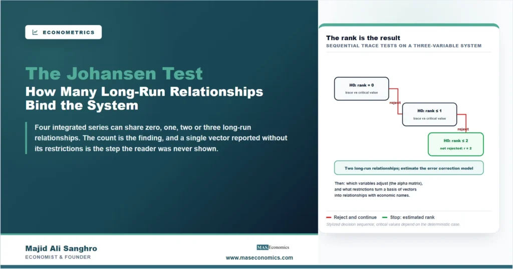
The trace statistic tests the null that the rank is at most r against the alternative that it is larger, using all the eigenvalues beyond the r-th. The maximum eigenvalue statistic tests the same null against the specific alternative that the rank is r plus one, using only the next eigenvalue. The procedure is sequential. Start with the null of no cointegration. If the statistic exceeds its critical value, reject and move to a rank of at most one; continue until the null is not rejected, and the rank at which the sequence stops is the estimate. The two statistics usually agree; when they do not, the trace is the more commonly reported and the disagreement is worth stating rather than hiding.
The critical values are not the familiar chi-squared ones. Because the variables have unit roots, the statistics have non-standard distributions that depend on how many variables are being tested and, more awkwardly, on which deterministic terms the model includes. Whether a constant or a trend sits inside the cointegrating relationship, outside it, or both changes the distribution and therefore the decision. Johansen distinguished five cases, and the choice among them is the most consequential setting in the whole procedure, because it is a statement about how the data behave in the long run.
| Case | Inside the cointegrating relationship | Outside it, in the short-run equation | What it assumes about the data |
|---|---|---|---|
| 1 | Nothing | Nothing | No drift, and the relationships pass through zero. Rarely credible for economic series |
| 2 | A constant | Nothing | The series have no trend, but the equilibrium has an intercept. Interest rates and ratios |
| 3 | A constant | A constant | The series trend linearly and the relationship among them does not. The usual choice for levels of money, prices and income |
| 4 | A constant and a trend | A constant | The series trend, and the equilibrium itself drifts. A trending combination such as a productivity-adjusted real wage |
| 5 | A constant and a trend | A constant and a trend | Quadratic trends in the levels. Almost never appropriate |

|
|||
Software defaults to the third case, and the default is right often enough to be dangerous, since choosing it for series that do not trend, or for a relationship that does, shifts the critical values and can change the estimated rank. The honest procedure is to plot the series, decide which case matches their behaviour, and say so. Where the choice is genuinely uncertain, Johansen also supplied a test that runs the rank determination jointly with the choice between adjacent cases.
Reading the Vectors, and the Matrix Most People Ignore
Once the rank is settled, the cointegrating vectors are estimated by maximum likelihood along with everything else, in one pass, which is the second advantage over the residual method and the reason the estimates are efficient in the sense our article on maximum likelihood estimation describes. But the vectors come out with a warning attached. A cointegrating vector is only defined up to a scale, so one coefficient is set to one and the others are read relative to it; and when the rank is two or more, any linear combination of the vectors is also a cointegrating vector, so the estimated ones are not unique. The software’s output is one basis for the space of long-run relationships, not the economic relationships themselves.
Turning a basis into economics requires restrictions. With two relationships among four variables, identifying each one needs at least one restriction beyond its normalisation, such as the requirement that the money demand relation excludes the interest rate or that the interest parity relation excludes income. Restrictions that come from theory can be imposed and then tested with a likelihood ratio statistic, which under the null has the chi-squared distribution that the rank tests lacked, so the machinery of our article on hypothesis testing applies. A rejected restriction is a finding about the theory. An unrestricted vector reported as if it were a demand equation is the most common misreading of the method.
The adjustment matrix is where the dynamics live, and it is routinely printed and ignored. Each row belongs to one variable and each entry says how much of last period’s disequilibrium in a given relationship that variable corrects this period. A negative and significant entry means the variable moves back toward the relationship; an entry that cannot be distinguished from zero means it does not. A variable whose entire row is zero never adjusts to any relationship: it is weakly exogenous, it drives the system rather than responding to it, and the test for that restriction is again a likelihood ratio. This is the long-run counterpart of the predictive ordering our article on Granger causality describes, and in a money demand system it answers whether money adjusts to income and prices or the reverse, which is often the substantive question the thesis began with.
What Goes Wrong in Practice
The procedure’s demands on the sample and on the specification are where results are won or lost, and the failures cluster into a few kinds.
The lag length comes first because everything else is conditional on it. Too few lags leave autocorrelation in the residuals, the rank tests then reject far too often, and a spurious relationship is found. Too many lags consume degrees of freedom that a system with four variables and a hundred observations cannot spare, and the tests lose power. The information criteria give different answers in short samples, the residual diagnostics are the arbiter, and the chosen lag belongs in the write-up alongside the reason. Related to it is sample size itself. The asymptotic critical values reject too readily in samples of the size macroeconomics usually has, so the trace statistic is often scaled by a small-sample factor of the kind Reinsel and Ahn proposed, and a rank found only without the correction is a rank found weakly.
The composition of the system matters in a way that surprises people. A stationary variable included among integrated ones is itself a cointegrating relationship of the trivial kind, a combination with a single non-zero weight, and it raises the estimated rank by one. A finding of two relationships among four variables where one variable was stationary is a finding of one relationship and one mistake. The unit root tests in our articles on stationarity and the augmented Dickey-Fuller test are therefore not optional preliminaries; every variable in the system has to be integrated of order one for the rank to mean what it is read to mean, which is also the requirement that the bounds procedure in our article on the ARDL bounds test was built to relax for single-equation work.
Structural change is the last and least tractable problem. A shift in the equilibrium relationship, of the kind our article on structural breaks catalogues, makes the combination non-stationary across the full sample even if it is stationary on either side of the break, and the test then finds no cointegration where there is some, or a vector that is an average of two. Johansen and co-authors extended the procedure to known break dates, and where a break is suspected the sub-sample results should be reported. Underneath all of these sits the assumption that the errors are normal and free of conditional heteroskedasticity. The rank tests are reasonably tolerant of departures; the likelihood ratio tests on the vectors and the adjustment matrix are less so, and those are the tests on which the economic conclusions rest.
MASEconomics Explains
3 concepts behind the Johansen procedure
These concepts are explored in depth across our educational articles library.
Conclusion
The Johansen test replaces a yes-or-no question with a count. Among a set of integrated variables it determines how many independent long-run relationships hold, estimates all of them at once from the system rather than one equation, and reports which variables do the adjusting when the system is pushed away from them. Each of those is something the residual-based approach cannot deliver, and together they are why the procedure is the standard tool for systems of three or more variables and for any question where the number of relationships is itself in doubt.
Its results are only as good as four decisions that precede them: the lag length, checked against the residuals rather than read off a criterion; the deterministic case, chosen to match how the series behave and stated; the composition of the system, with every variable confirmed to have a unit root; and the identifying restrictions that turn a basis of vectors into relationships with economic names. Report the trace and maximum eigenvalue statistics with their critical values, the vectors with the restrictions imposed and tested, and the adjustment coefficients with the weak exogeneity tests, and the reader can see what the data supported. Report a single normalised vector as if it were the money demand equation, and the reader is being asked to take the most important step on trust.
Frequently Asked Questions
What does the Johansen test actually test?
The number of cointegrating relationships among a set of integrated variables, which is the rank of the matrix on the lagged levels in the vector error correction model. It proceeds sequentially, testing a rank of zero, then at most one, and so on, until the null is not rejected. The rank at which it stops is the estimated number of long-run relationships.
What is the difference between the trace and maximum eigenvalue statistics?
Both test the null that the rank is at most r. The trace statistic uses all the remaining eigenvalues and tests against the alternative that the rank is larger than r; the maximum eigenvalue statistic uses only the next eigenvalue and tests against the specific alternative of rank r plus one. They usually agree, and when they do not the disagreement should be reported rather than resolved by choosing the convenient one.
When is Johansen preferred to Engle-Granger?
When there are more than two variables and several long-run relationships may exist, since the residual method can find at most one and its result depends on which variable is normalised. Johansen also estimates the relationships and the adjustment coefficients jointly by maximum likelihood, which is more efficient than a two-step procedure. It needs a longer sample to estimate the system reliably.
Why does the choice of deterministic case matter so much?
Because the critical values of the rank tests depend on whether a constant or trend sits inside the cointegrating relationship, outside it, or both. Choosing a case that does not match the data’s behaviour shifts the critical values and can change the estimated rank. The case should be chosen by inspecting the series, and it should be stated with the results.
Can a cointegrating vector be read as a structural equation?
Not without restrictions. When the rank is two or more, any combination of the estimated vectors is also a cointegrating vector, so the output is a basis rather than a set of economic relationships. Identifying restrictions from theory must be imposed on each vector and tested with a likelihood ratio statistic before a vector can be given an economic name.
What does weak exogeneity mean in a Johansen system?
That a variable does not adjust to any of the long-run relationships, which shows up as a row of zeros in the adjustment matrix. Such a variable drives the system’s long run rather than responding to it, and the restriction can be tested with a likelihood ratio test. In a money demand system it answers whether money adjusts to income and prices or the reverse.
Thanks for reading! The count is the finding, and a single vector reported without its restrictions is the step the reader was never shown. Happy learning with MASEconomics