The Taylor Rule Reaction Function: Estimation and Limitations

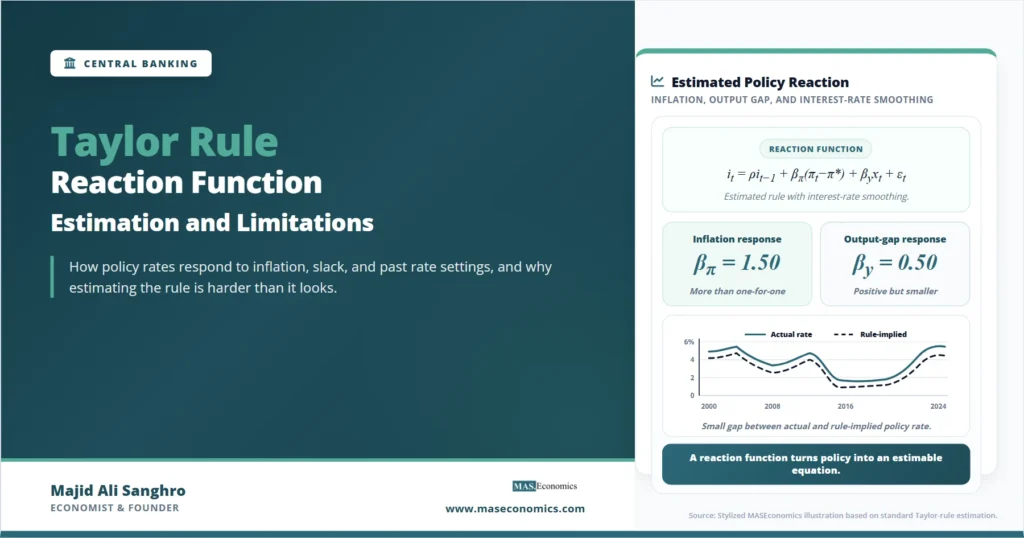
In 1993, John Taylor showed that a simple interest-rate rule could describe much of Federal Reserve behavior during a period of relatively stable US monetary policy. The Taylor rule reaction function takes that insight one step deeper: it asks how a central bank appears to adjust its policy rate when inflation, economic slack, and its own past decisions change.

The original Taylor Rule is usually presented as a benchmark formula. A reaction function is more empirical. It turns that benchmark into an estimated policy equation, using data to infer how strongly a central bank reacts to inflation, output gaps, unemployment gaps, financial stress, or exchange-rate pressure. That makes it useful for research, but also risky if the data, timing, or identification strategy are weak.

This distinction matters because monetary policy is not observed as a clean laboratory experiment. The policy rate moves because central banks respond to the economy, but the economy also responds to expected policy. Inflation, output, unemployment, and interest rates are jointly determined. A regression that looks simple on paper can therefore hide serious problems of endogeneity, real-time data uncertainty, omitted variables, and regime change.

Taylor Rule Reaction Function Form

A Taylor rule reaction function is an equation that links a central bank’s policy instrument, usually a short-term nominal interest rate, to the economic conditions that policymakers are assumed to care about. The standard Taylor-style rule can be written as:

Baseline Taylor-Style Rule

The policy rate responds to the neutral real rate, current inflation, the inflation gap, and the output gap.

Here, \(i_t\) is the nominal policy rate, \(r_t^*\) is the neutral real interest rate, \(\pi_t\) is inflation, \(\pi^*\) is the inflation target, and \(y_t – y_t^*\) is the output gap. The coefficients \(\phi_\pi\) and \(\phi_y\) measure how strongly policy responds to inflation and real activity.

In Taylor’s original Discretion versus Policy Rules in Practice, the benchmark values were simple and transparent: a long-run real rate of 2 percent, an inflation target of 2 percent, and reaction coefficients of 0.5 on both the inflation gap and output gap. The rule implied that when inflation rises one percentage point above target, the nominal policy rate rises by more than one percentage point because the rate also includes inflation itself.

An estimated reaction function is different. It does not impose the coefficients from the benchmark rule. Instead, it asks what values best fit observed central bank behavior. Researchers often estimate a version like this:

Estimated Reaction Function

The lagged policy rate captures interest-rate smoothing; \(x_t\) may be an output gap, unemployment gap, or another activity measure.

The lagged interest rate \(i_{t-1}\) is important because central banks rarely move policy rates in abrupt jumps unless financial conditions force them to. A high value of \(\rho\) suggests interest-rate smoothing: policymakers move gradually toward a desired rate instead of adjusting fully in one meeting. This connects the Taylor rule to broader articles on monetary policy tools and monetary policy lags, where timing and transmission are central.

Interpreting Estimated Coefficients

The inflation coefficient is the most closely watched parameter. A central bank that raises the nominal policy rate by more than one-for-one when inflation increases is often said to satisfy the Taylor principle. In simple New Keynesian models, this kind of reaction can help stabilize inflation expectations because it raises the real interest rate when inflation moves above target.

The output-gap or unemployment-gap coefficient captures the real-side part of the reaction function. A positive output-gap coefficient means the central bank raises rates when output is above potential and lowers rates when output is below potential. In a dual-mandate framework, this real-side response is not a departure from inflation control. It is part of stabilizing the economy when demand is too strong or too weak.

The smoothing coefficient is often misunderstood. It does not necessarily mean policymakers are timid. It may reflect uncertainty about incoming data, concern about financial-market disruption, committee decision-making, or a deliberate attempt to communicate a predictable path. The same coefficient can therefore represent several different institutional mechanisms.

Table 1. Interpreting Taylor Rule Reaction Function Parameters

Parameter	Common Interpretation	Research Risk	Policy Reading
\(\beta_\pi\)	Response to the inflation gap	Inflation may be endogenous to expected policy	Higher values suggest stronger inflation stabilization
\(\beta_y\)	Response to the output or unemployment gap	Slack is unobservable and heavily revised	Higher values suggest greater concern for real activity
\(\rho\)	Interest-rate smoothing	May reflect omitted variables rather than deliberate gradualism	Higher values imply slower adjustment to the desired rate
\(\alpha\)	Intercept or long-run rate component	Blends the neutral rate, inflation target, and sample average	Hard to interpret without structural assumptions
Core lesson	The coefficient estimates are not mechanical measures of central-bank preferences. They depend on timing, data vintage, model specification, and identification.
Source: MASEconomics editorial synthesis based on Taylor (1993), Clarida, Galí, and Gertler (2000), and Orphanides (2001).

Estimating the Reaction Function

The simplest approach is ordinary least squares. A researcher collects observations on the policy rate, inflation, and an output-gap measure, then estimates the coefficients that minimize squared errors. For a first pass, this resembles the logic behind simple regression and multiple regression.

But a Taylor rule is rarely a clean static regression. Monetary policy is forward-looking, persistent, and shaped by expectations. Policymakers respond not only to current inflation but also to expected inflation. They care about forecast errors, financial stability, exchange-rate pressure, and risks that may not appear in a simple equation. As a result, many estimated reaction functions use expected inflation, lagged variables, or instrumental variables.

A common forward-looking specification follows the spirit of Richard Clarida, Jordi Galí, and Mark Gertler’s Monetary Policy Rules and Macroeconomic Stability. Their approach estimates how the policy rate responds to expected inflation and expected real activity, rather than only to realized data. This matters because a central bank setting rates in March does not know next year’s inflation with certainty. It acts on forecasts, models, staff projections, and risk assessments.

The econometric challenge is that expected inflation is not directly observed. Researchers may use survey expectations, central-bank forecasts, market-implied measures, or lagged data as instruments. Each choice changes the meaning of the coefficient. A forecast-based rule is closer to what policymakers may have seen at the time. A revised-data rule is closer to what later researchers know with hindsight.

Real-Time Data Problem

Athanasios Orphanides made the real-time data problem central to Taylor rule research. In Monetary Policy Rules Based on Real-Time Data, he showed that policy prescriptions can differ sharply when researchers use the data available to policymakers at the time rather than later-revised data. The problem is especially severe for the output gap.

The output itself is revised. Potential output is estimated. The output gap is the difference between an observed variable that can change with revisions and an unobserved benchmark that is model-dependent. A central bank may appear to have ignored a rule when judged by today’s revised data, even if the real-time data available at the meeting gave a different signal.

This is one reason reaction functions are not the same as audit tools. They can help researchers compare policy regimes, but they should not be treated as a mechanical scorecard for a single meeting. The measurement problem is much less visible in a basic presentation of the Taylor Rule, but it becomes decisive once the rule is estimated.

The same issue appears in inflation measurement. A rule estimated with CPI inflation may differ from one estimated with PCE inflation. For the United States, the Federal Reserve’s preferred inflation measure is tied to the personal consumption expenditures price index, which is why a reader comparing reaction functions should also understand the PCE index. The choice of headline inflation, core inflation, expected inflation, or trimmed inflation changes the estimated response.

Identification Challenges

A reaction function can fit the data and still fail to identify the causal policy rule. Identification asks whether the coefficient being estimated actually captures the structural response of policymakers, rather than a statistical correlation created by simultaneous movements in the economy.

Suppose inflation rises and the central bank raises the policy rate. The regression may show a positive inflation coefficient. But the size of that coefficient depends on why inflation rose, what policymakers expected to happen next, how markets anticipated the move, and whether output was already slowing. The observed interest rate is part of an equilibrium, not an isolated treatment.

John Cochrane’s Identification with Taylor Rules: A Critical Review argues that Taylor rule estimates can be fragile because the same data may be consistent with different equilibrium interpretations. This is not a reason to discard reaction functions. It is a reason to treat them as evidence that depends on a model, not as self-contained proof of how monetary policy works.

Instrumental variables can help when the policy variable or inflation variable is endogenous, but instruments are difficult to justify. Valid instruments must affect the policy-rate decision through the intended channel and not through omitted macroeconomic shocks. That is a demanding requirement in monetary economics. The logic is similar to the problem discussed in instrumental variables, where a plausible instrument must be both relevant and exogenous.

Policy Inertia and Long-Run Response

When a lagged interest rate appears in the equation, the short-run coefficient and the long-run coefficient are not the same. Suppose the estimated rule is:

Long-Run Reaction

When \(\rho\) is high, a small short-run response can imply a much larger eventual adjustment.

This distinction is central. A central bank may raise rates slowly, but the implied long-run response may still be large if it keeps moving in the same direction over several meetings. Conversely, a model may estimate a high smoothing coefficient because it omits financial stress, exchange-rate pressure, or changes in the neutral rate. In that case, the lagged interest-rate term absorbs missing information.

For research, the smoothing term is useful but dangerous. It improves fit, but it can also blur the line between deliberate gradualism and omitted-variable bias. Researchers, therefore, often compare several specifications: with and without smoothing, with different slack measures, and across different sample periods.

Regime Change Instability

Central bank behavior is not fixed forever. A reaction function estimated over one regime may fail in another. The Volcker disinflation, the zero lower bound after 2008, the inflation surge after the pandemic, and the return of balance-sheet policy all changed the environment in which interest-rate rules operated.

Clarida, Galí, and Gertler’s research is influential partly because it compares different monetary-policy regimes. Their findings are often interpreted as evidence that the post-1979 Federal Reserve reacted more strongly to expected inflation than the pre-Volcker Fed. That interpretation connects reaction-function estimates to the broader history of credibility, inflation targeting, and inflation expectations.

But regime comparison creates its own risk. A coefficient estimated before the global financial crisis may not describe policy at the effective lower bound. A coefficient estimated during inflation targeting may not describe policy under average inflation targeting. A coefficient estimated for the United States may not transfer to an emerging market central bank facing exchange-rate pressure and capital-flow volatility.

This is where structural breaks become central. A reaction function should be tested across subperiods, not simply estimated over the longest possible sample. More data is not always better if the sample combines incompatible regimes.

Measuring Economic Slack

The output gap is conceptually attractive but empirically difficult. It asks how far actual output is from potential output. Potential output, however, is not observed. Different methods produce different gaps: production-function estimates, statistical filters, multivariate filters, and official estimates from institutions such as the Congressional Budget Office.

Some reaction functions use the unemployment gap instead: the difference between actual unemployment and an estimate of the natural rate. This can be easier to communicate, but it has the same unobserved-benchmark problem. The natural rate changes over time and is revised as economists learn more about labor-market participation, matching efficiency, demographics, and productivity.

The choice matters. A central bank may look too loose or too tight depending on whether slack is measured through output, unemployment, capacity utilization, or a broader labor-market index. This is one reason Taylor rule estimates should be interpreted as conditional on the slack measure, not as independent facts.

Forward-Looking Rules and Expectations

Modern central banks often describe policy in forward-looking terms. They set rates based on where inflation is expected to go, not only where inflation has been. That is sensible for policy because interest-rate decisions affect the economy with a lag. It is difficult to estimate because expectations are hard to measure and may already include beliefs about future policy.

For example, market-based inflation expectations may fall after investors anticipate that the central bank will tighten. If a researcher then uses those expectations in a reaction function, the estimated policy response may understate the central bank’s true anti-inflation stance. The expectation variable is not independent of the policy rule. It is partly created by it.

This is why reaction-function estimation often belongs closer to macroeconometrics than to simple descriptive statistics. Vector autoregressions, narrative shocks, high-frequency event studies, and model-based identification strategies can help isolate monetary-policy surprises, although each brings its own assumptions. Readers interested in dynamic systems can connect this issue to VAR impulse responses.

Taylor Rule as a Policy Benchmark

Central banks do not usually promise to follow a Taylor rule mechanically. The Federal Reserve’s Statement on Longer-Run Goals and Monetary Policy Strategy emphasizes the goals of maximum employment and stable prices, while leaving room for judgment across a broad range of economic conditions. That institutional reality matters for estimation.

A rule-implied rate can be useful as a benchmark. It helps ask whether the policy looks unusually loose or tight relative to a simple historical pattern. It can discipline policy debate by forcing the analyst to state assumptions about inflation, slack, and the neutral rate. The Atlanta Fed’s Taylor Rule Utility shows how different assumptions can generate different prescriptions from the same basic framework.

But a benchmark is not a legal command. A central bank may deviate because financial markets are impaired, the banking system is under stress, the neutral rate has shifted, inflation is supply-driven, or the policy rate is constrained by the lower bound. During such periods, balance-sheet tools, lending facilities, and communication may matter as much as the short-term policy rate. This is why reaction functions should be read alongside broader coverage of central banking and monetary policy.

Common Estimation Mistakes

The first mistake is treating revised data as if it were the real-time information set. This can make historical policymakers look irrational when they were responding to the data they actually had. The second mistake is treating the output gap as known. It is an estimate, and often a fragile one.

The third mistake is ignoring the interest-rate smoothing term. Without \(i_{t-1}\), the estimated reaction may exaggerate short-run responses. With \(i_{t-1}\), the estimate may hide omitted variables. Both versions should be interpreted carefully.

The fourth mistake is estimating one rule over a long sample without checking for regime shifts. Monetary policy under high inflation, at the lower bound, and during a credibility-building phase may follow different patterns. A single coefficient can average across very different policy environments.

The fifth mistake is confusing statistical fit with policy explanation. A high \(R^2\) does not prove that the equation captures the central bank’s true reaction function. Interest rates are persistent, inflation is persistent, and macroeconomic variables move together. Good in-sample fit can come from persistence rather than deep economic structure.

Interpreting Taylor Rule Estimates

A careful reading starts with the information set. Are the inflation and slack variables real-time or revised? Are expectations measured through forecasts, surveys, market prices, or lagged values? Is the sample period stable, or does it cross major regime breaks?

Next, examine the coefficient units. A response to the inflation gap is not the same as a response to the inflation level. A response to unemployment may have the opposite sign from a response to output. A short-run response in a smoothing model must be translated into a long-run response before making claims about the Taylor principle.

Then ask whether the equation includes relevant omitted variables. A small open economy may respond to exchange rates. A central bank under financial stress may respond to credit spreads. A lower-bound episode may require shadow rates or balance-sheet variables. An estimated reaction function is always a simplified map of policy behavior, not the full policy process.

Explains

Conclusion

The Taylor rule reaction function is powerful because it converts a familiar monetary-policy benchmark into an empirical question: how does the central bank appear to move its policy rate when inflation and real activity change? That question is useful for comparing regimes, testing policy narratives, and organizing debate about whether policy was tight or loose relative to a simple rule.

Its limitations are just as important. Coefficients depend on real-time data, expectations, slack estimates, sample periods, and identification assumptions. A reaction function that fits the data may still fail to identify the central bank’s structural rule. A rule-implied rate may clarify the debate, but it does not replace judgment, institutional context, or the broader set of monetary-policy tools.

The best use of the Taylor rule reaction function is therefore disciplined comparison, not mechanical prescription. It is a way to ask sharper questions about central bank behavior while remaining honest about the uncertainty inside every estimated policy rule.

Frequently Asked Questions

Thanks for reading! If you found this helpful, share it with friends and spread the knowledge. Happy learning with MASEconomics