Ridge Lines Isoquant: Economic Region of Production

A production manager can add more labor to a fixed set of machines and raise output for a while, but after congestion sets in, extra workers may reduce total output. The same logic can apply to capital when too many machines are crowded into a limited workspace. Ridge lines isoquant analysis marks the boundary between input combinations that make economic sense and combinations where one input has become counterproductive.

Ridge lines matter because an isoquant map contains more than technically feasible combinations. Some parts of the map show input mixes where output can be held constant only by adding more of both inputs, which means one input has a negative marginal product. Those regions are technically drawable, but they are not economically rational for a cost-minimizing firm.

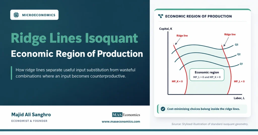
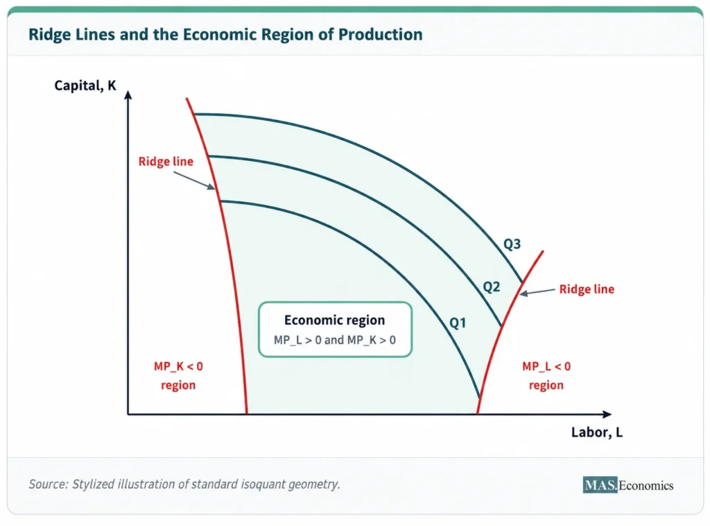
In producer theory, the useful part of an isoquant map is called the economic region of production. It is the zone where labor and capital both have positive marginal products, isoquants slope downward, and cost-minimizing choices can be found with ordinary isocost logic.

Ridge lines mark production boundaries

Ridge lines are curves drawn through special points on a family of isoquants. Each ridge line connects points where one input’s marginal product is zero. Inside the two ridge lines, both inputs have positive marginal products. Outside them, at least one input has become so excessive relative to the other input that adding more of it reduces output.

For a two-input production function, output can be written as:

Here, \(Q\) is output, \(K\) is capital, and \(L\) is labor. An isoquant shows all combinations of \(K\) and \(L\) that produce the same level of output. The broader logic belongs to the study of production functions and isoquant curves, but ridge lines focus on a narrower question: which parts of the isoquant map should a rational producer actually use?

The answer depends on marginal products. The marginal product of labor is \(MP_L = \partial Q / \partial L\), and the marginal product of capital is \(MP_K = \partial Q / \partial K\). The economic region exists where both are positive:

Economic Region

Both inputs add to output at the margin inside the economic region of production.

If \(MP_L = 0\), extra labor no longer increases output at that point. If \(MP_K = 0\), extra capital no longer increases output at that point. The ridge lines trace these zero marginal product conditions across different output levels.

Isoquant slopes reveal marginal products

The slope of an isoquant is the marginal rate of technical substitution. It measures how much capital can be reduced when labor rises while output stays unchanged. With labor on the horizontal axis and capital on the vertical axis, the slope of an isoquant is:

Isoquant Slope

This formula explains why ridge lines matter. When \(MP_L > 0\) and \(MP_K > 0\), the isoquant slopes downward. More labor can replace some capital while keeping output constant. This is the normal substitution region used in producer theory.

When one marginal product becomes negative, the isoquant can bend backward or slope upward. An upward-sloping isoquant segment means output can be kept constant only by adding more of both inputs. That is not a sensible production choice because one input is doing harm at the margin.

A firm minimizing cost will not choose a point where \(MP_L < 0\). Reducing labor would lower cost and raise output, so the original point cannot be efficient. The same reasoning applies when \(MP_K < 0\). Reducing capital would lower cost and raise output. Ridge lines therefore separate technically possible points from economically relevant points.

The economic region keeps inputs productive

The economic region of production is the area between the two ridge lines. In this region, labor and capital both raise output at the margin. Isoquants slope downward, and a firm can substitute labor for capital or capital for labor without entering a wasteful input range.

This does not mean every point inside the economic region is cost minimizing. It means only that the point is economically admissible. Cost minimization requires the firm to compare the isoquant with input prices, usually through an isocost line. The ridge lines answer the prior question of whether the input combination belongs to the meaningful part of the technology.

Inside the economic region, the firm can use ordinary substitution logic. If labor becomes cheaper relative to capital, the firm may move toward a more labor-intensive point on the same isoquant. If capital becomes cheaper relative to labor, the firm may move toward a more capital-intensive point. This is the same input-price logic developed in the isocost line framework.

Outside the ridge lines, price changes are not the central issue. A firm would first remove the input with negative marginal product. No positive wage or rental price can justify paying for an input that reduces output at the margin when less of that input would be cheaper and more productive.

Table 1. Production regions in an isoquant map

Region	Marginal product condition	Isoquant shape	Economic interpretation
Inside ridge lines	\(MP_L > 0\), \(MP_K > 0\)	Downward sloping	Economically relevant input substitution
Beyond labor ridge	\(MP_L < 0\)	Backward or upward segment	Labor is excessive at the margin
Beyond capital ridge	\(MP_K < 0\)	Backward or upward segment	Capital is excessive at the margin
Cost-minimizing search zone	\(MP_L > 0\), \(MP_K > 0\)	Convex, downward-sloping segment	Candidate zone for producer equilibrium
Source: MASEconomics editorial synthesis based on standard producer theory.

Cost minimization rejects upward isoquant segments

Cost minimization begins with a target level of output and a set of input prices. The firm looks for the lowest-cost combination of labor and capital capable of producing that output. On a well-behaved part of an isoquant map, this occurs where an isoquant is tangent to an isocost line.

The tangency condition can be written as:

Cost-Minimizing Tangency

The marginal rate of technical substitution equals the input price ratio.

Here, \(w\) is the wage rate and \(r\) is the rental price of capital. The condition is meaningful only when both marginal products are positive. If one marginal product is negative, the ratio no longer describes a sensible trade-off between inputs. It describes a region where one input should be reduced, not substituted at the margin.

This is why ridge lines support the logic of costs of production. Costs are not minimized by every technically feasible input bundle. They are minimized only among combinations that produce the target output without wasting an input. The ridge lines remove the wasteful parts of the isoquant map before the isocost line selects the least-cost point.

The same distinction appears in producer equilibrium. A tangency between an isoquant and an isocost line is economically valid only if it occurs within the ridge lines. A formal tangency outside the economic region would fail the basic test of positive marginal productivity.

Ridge lines differ from expansion paths

Ridge lines and expansion paths both appear on isoquant maps, but they answer different questions. Ridge lines define the boundary of the economic region. An expansion path traces the sequence of least-cost input choices as output changes.

The ridge lines are technology boundaries. They are determined by the shape of the production function and the points where one marginal product becomes zero. They do not depend on wages or rental rates. A change in input prices does not move the ridge lines unless the underlying technology changes.

The expansion path depends on both technology and input prices. It connects the cost-minimizing tangency points across output levels. A change in the wage-rental ratio can rotate isocost lines and shift the expansion path even when the ridge lines stay fixed. This makes the expansion path a cost-minimization curve, not a boundary of feasible economic production.

A useful way to separate the two concepts is to treat ridge lines as excluding bad choices and the expansion path as selecting the best choices from the remaining good region. Ridge lines say where rational production can occur. The expansion path says which points a cost-minimizing firm chooses as scale changes.

Examples show the boundary logic

Consider a workshop with five machines and one worker. Adding another worker may raise output because the machines are underused. Adding more workers can continue to raise output until congestion begins. At some point, extra workers may block movement, wait for the same tools, and reduce the average coordination of the workshop. Once the marginal product of labor reaches zero, the labor ridge line has been reached for that output level.

The opposite case can occur when capital becomes excessive. A firm may add machines to help workers produce more, but too many machines in a limited space can create bottlenecks, maintenance delays, and idle capacity. If an additional machine reduces output by crowding the production floor, the marginal product of capital has become negative. The capital ridge line marks the boundary before that region begins.

These examples are not claims that firms commonly operate where marginal products are negative. They explain why the theoretical boundary matters. A production function can describe a wide technical surface, but rational cost minimization uses only the part of that surface where each input is productive at the margin.

This caveat also clarifies why some introductory treatments skip ridge lines. In simple examples, isoquants are often drawn only in the downward-sloping, convex region. That picture is useful for teaching substitution, but it hides the broader map from which the economic region has already been selected.

Some production functions need no ridge lines

Not every production function generates a visible ridge-line problem. A standard Cobb-Douglas production function with positive exponents usually has positive marginal products for positive input levels:

In that case, adding more labor or capital raises output, although possibly at a diminishing rate. The isoquants do not normally bend into a region where one input has negative marginal product. The economic region is effectively the relevant positive input space, so ridge lines are not central to the analysis.

Other technologies can generate stronger congestion effects or managerial limits. In those cases, marginal products can turn negative after one input becomes excessive. Ridge lines then become a useful device for separating feasible production from economically meaningful production.

The broader lesson is that ridge lines are not decorative curves. They appear when the production technology has regions that should be excluded from cost-minimizing analysis. They keep the model focused on input combinations where substitution is meaningful, and both inputs contribute positively to output.

Explains

Conclusion

Ridge lines isoquant analysis identifies the economically relevant part of an isoquant map by locating where marginal products stop being positive. The two ridge lines form boundaries around the economic region of production, where isoquants slope downward, and both labor and capital add to output at the margin.

This distinction matters for cost minimization. An isocost line can select a least-cost input bundle only after the wasteful parts of the isoquant map have been excluded. Ridge lines therefore work as a filter before producer equilibrium analysis begins.

The concept is most useful for technologies where excessive labor or excessive capital can reduce output. In simpler production functions with positive marginal products over the relevant range, ridge lines may remain implicit. The underlying rule is the same: rational production belongs in the region where every paid input contributes positively at the margin.

Frequently Asked Questions

Thanks for reading! If you found this helpful, share it with friends and spread the knowledge. Happy learning with MASEconomics