Inflation Persistence: Why Past Inflation Drives Future Inflation

When US core PCE inflation peaked at 5.6 percent in February 2022 and then took nearly three years to settle near 2.7 percent by late 2024, the slow descent raised the question of whether the disinflation reflected the predictable echo of supply shocks or stickier-than-expected behavior. The answer turns on a property of inflation dynamics that has its own name in macroeconomics: inflation persistence. Persistence measures the degree to which past inflation predicts future inflation, holding other drivers constant. A persistent inflation series adjusts slowly to new information. A non-persistent series adjusts quickly. The distinction is not academic. It changes how central banks set policy, how forecasters build models, and how households and firms read incoming data.

Measuring Inflation Persistence

Persistence describes the speed at which a time series returns to its mean after a shock. In inflation terms, it measures how much of last quarter’s deviation from trend carries into this quarter’s inflation. A simple way to formalize it uses an autoregressive specification. In its first-order form, inflation depends on its own lagged value plus a shock:

\( \pi_{t} \) is inflation in period \( t \), \( \rho \) is the persistence coefficient, and \( \varepsilon_{t} \) is the shock. A \( \rho \) close to zero means inflation forgets the past quickly. A \( \rho \) close to one means inflation is highly persistent and shocks decay slowly. A \( \rho \) of exactly one would imply a unit root, where shocks never decay.

The empirical literature usually generalizes this to higher-order autoregressions or to the sum of autoregressive coefficients in an AR(p) specification. The sum, sometimes denoted \( \hat{\rho} \), provides a single summary statistic for persistence that is comparable across samples, countries, and inflation measures. As time series econometrics shows, this framework lets researchers ask a precise question: how much memory does the inflation process carry?

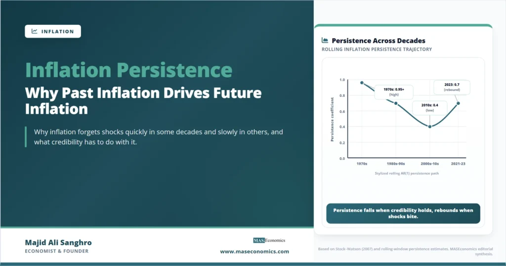
The answer turns out to depend on the period. Robert Stock and Mark Watson, in their influential survey “Why Has US Inflation Become Harder to Forecast?” (2007), documented that the sum of AR coefficients on US inflation hovered close to one through the 1970s and early 1980s, declined sharply over the late 1980s and 1990s, and remained low through the mid-2000s. The implication was striking. The same statistical question, asked of the same country, returned very different answers in different decades.

Sources of Inflation Persistence

Persistence does not have a single mechanism. It can arise from at least two distinct sources, and they require very different policy responses.

The first source is intrinsic persistence, also called backward-looking or indexation-driven persistence. It comes from price- and wage-setting institutions that mechanically tie current price changes to past inflation. Cost-of-living adjustment clauses in labor contracts, multi-year fixed-price commercial contracts, regulated tariffs that update on a lag, and rent renewal cycles all produce intrinsic persistence. When past inflation is encoded in the institutional architecture, inflation today depends on inflation yesterday for reasons that have nothing to do with what the economy is doing now.

The second source is expectations-driven persistence. If households, firms, and wage-setters use past inflation to forecast future inflation, then they will set prices and wages today based on what they observed yesterday. Expectations-driven persistence vanishes when expectations are well anchored at a credible inflation target, because the forecasting rule shifts from “extrapolate the past” to “expect the target.” This distinction maps directly onto the inflation expectations framework: backward-looking expectations create persistence; forward-looking, target-anchored expectations destroy it.

Why does this distinction matter? Because the policy implication depends on the source. If persistence is intrinsic, central banks must wait for institutional contracts to unwind. If persistence is expectations-driven, a credible policy framework can collapse it quickly. The same observed AR coefficient implies different costs of disinflation depending on what is generating it. The Atlanta Fed’s Sticky-Price CPI measure, which separates price categories that change infrequently from those that change often, is one direct attempt to operationalize the institutional channel of persistence.

Great Moderation Decline in Persistence

Stock and Watson, James Cogley and Thomas Sargent (2002), and Jeffrey Fuhrer (2010) documented a coherent finding that has shaped how the literature thinks about persistence today. The persistence of US inflation fell sharply between the early 1980s and the early 1990s. Estimates of \( \hat{\rho} \) for headline and core CPI dropped from near unity to around 0.4 to 0.6 depending on the inflation measure and the lag specification. The shift was statistically detectable through standard structural break tests and was robust to different filters and trend assumptions.

Three explanations dominate the literature. The first is monetary policy regime change. The Volcker disinflation established that the Federal Reserve was willing to incur output costs to bring inflation down, and the subsequent commitment to low and stable inflation under Greenspan and Bernanke gave households and firms a focal point for expectations. As inflation targeting spread across advanced economies, the expectations-driven source of persistence collapsed.

The second is institutional change. Cost-of-living adjustment clauses in US private-sector contracts had largely disappeared by the mid-1980s. Union density declined. Italy’s scala mobile indexation system was abolished in 1992. The intrinsic, indexation-driven source of persistence shrank at the same time.

The third is the changing nature of shocks. The 1970s combined a series of large supply shocks (two oil crises, food-price surges, productivity slowdown) with monetary accommodation. The Great Moderation period of 1985 to 2007 had smaller, more transitory shocks. Less persistent shocks produce less persistent inflation, even with the same structural transmission.

The empirical literature has not settled on a single ranking among the three. But the convergence of evidence from the Führer’s work at the Boston Fed and the IMF’s persistence studies suggests that monetary regime credibility is doing the largest share of the work.

Table 1. Estimated US Inflation Persistence Across Sub-Samples

Sample period	Inflation measure	Sum of AR coefficients (\(\hat{\rho}\))	Interpretation
1960–1983	Core CPI	0.95–1.00	Near-unit-root, very high persistence
1984–1999	Core CPI	0.55–0.70	Moderate, post-Volcker decline
2000–2019	Core CPI	0.35–0.50	Low; well-anchored Great Moderation
2020–2024	Core CPI	0.55–0.75	Rebound during pandemic-era surge
1960–1983	Core PCE	0.90–0.98	Comparable to CPI in pre-1984 sample
2000–2019	Core PCE	0.30–0.45	Slightly lower than CPI counterpart
Structural break	Multiple measures	around 1984	Detected by Stock–Watson and Cogley–Sargent
Source: Stock and Watson (2007), NBER WP 12324; Cogley and Sargent (2002); Fuhrer (2010), Boston Fed FEDS 2009-33; BLS and BEA inflation series. Ranges reflect published estimates across lag-length and trend specifications.

2021–2024 Persistence Rebound

The pandemic-era inflation surge revived a question that had been mostly dormant for two decades. Rolling-window estimates of US inflation persistence, using either core CPI or core PCE, rose noticeably from 2020 through 2023. Several IMF and Federal Reserve research papers documented the rebound. The sum of AR coefficients on US core inflation, estimated over rolling 10-year windows, climbed from roughly 0.4 in the late 2010s to around 0.6 to 0.7 by 2023, before easing as headline pressures normalized.

US Inflation Persistence: Rolling 10-Year Window

Stylized illustration based on Stock–Watson (2007), Cogley–Sargent (2002), and Fuhrer (2010) rolling-window persistence estimates of US core inflation. Levels and shape approximate; trajectory meant to convey the historical pattern.

Three reasons explain the rebound. The first is composition. Service-price inflation, which has historically been the most persistent component of the inflation basket, rose disproportionately during 2022 and 2023 even as goods inflation faded. As sticky services inflation dynamics show, the residual mile of disinflation runs through wage-sensitive service prices that adjust slowly. A higher weight on persistent components mechanically raises the measured persistence of the overall index.

The second is shock size. Even when the structural persistence of inflation is low, large shocks produce long-lived effects in absolute terms. The energy and supply-chain shocks of 2022 were large enough that even with modest pass-through coefficients, the cumulative inflation response stretched well into 2024. This shows up in rolling-window estimates as elevated persistence, but it can reflect shock magnitude rather than any change in the underlying transmission mechanism.

The third is partial unanchoring of short-run expectations. While long-run inflation expectations from the New York Fed Survey of Consumer Expectations and the University of Michigan survey stayed within their pre-pandemic range, one-year expectations briefly exceeded 6 percent in 2022. The temporary unanchoring at short horizons reintroduced an expectations-driven persistence channel that had been dormant during the Great Moderation. As short-run expectations normalized, the persistence rebound began to fade.

Implications for Forecasting and Policy

The practical stakes of inflation persistence run through three channels. Each one shifts policy choices when persistence rises or falls.

The first is the inflation forecast. Standard forecasting models, including the Federal Reserve’s FRB/US model and the IMF’s World Economic Outlook framework, treat inflation as a partly autoregressive process. The implied persistence directly affects how long inflation is projected to deviate from target after a shock. A persistence coefficient of 0.4 implies that half of an inflation shock dies out in less than one year. A persistence coefficient of 0.8 implies it takes more than three years. The same observed inflation deviation produces very different forecasts depending on the assumed \( \hat{\rho} \).

The second is the cost of disinflation. The relationship between persistence and the Phillips Curve trade-off is direct. When inflation persistence is high, more output must be lost to bring inflation down because the inflation response to slack is slower. This is the persistence component of the sacrifice ratio. Studies of disinflation episodes in the 1980s, when persistence was high, find sacrifice ratios above one. Disinflation episodes during the inflation-targeting era, when persistence is low, often produce smaller losses.

The third is the appropriate aggressiveness of policy response. Under a Taylor-rule framework, a central bank that knows inflation is highly persistent must respond more aggressively to a given inflation deviation, because that deviation will not fade on its own. Under low persistence, the same deviation may be self-correcting and warrants a more measured response. The challenge is that persistence is not observable in real time. Central banks must infer it from rolling-window estimates that are themselves noisy and can change with the next shock.

Asymmetry of Persistence Estimates

One of the most important findings in the persistence literature is that estimates depend heavily on assumptions about the trend and the sample. A constant-mean specification on a sample that includes both the high-inflation 1970s and the low-inflation 2000s will misattribute the change in mean to high persistence. The standard solution, used by Cogley and Sargent and adopted in most subsequent work, is to allow the inflation mean to follow a slow stochastic process or to estimate persistence around a time-varying trend. When this is done properly, the AR coefficients on the cyclical component of inflation are typically smaller than the headline AR coefficients on the raw series.

This is not just a statistical nuance. It affects what the persistence number means for policy. If the apparent persistence in a long sample is mostly about a slow drift in the inflation target, then policy credibility is the variable doing the work. If the persistence is in the cyclical fluctuations around a stable trend, then institutional and expectational channels are at play. Distinguishing the two is what makes serious persistence work harder than simply running an AR(p) regression on the raw series. The Phillips Curve and persistence literatures intersect here: a flatter Phillips Curve, as documented in many post-2000 studies, is observationally similar to lower persistence, and disentangling them requires modeling both jointly. As the Phillips Curve framework and its New Keynesian variants suggest, the slope of the trade-off and the persistence of inflation move together when expectations re-anchor.

Explains

Conclusion

The inflation persistence framework remains one of the most useful organizing tools in modern macroeconomic analysis because it gives a single, comparable measure of how inflation responds to its own past. The historical record across advanced economies is consistent. Persistence was high in the 1970s and early 1980s, when inflation expectations were unanchored, and indexation was widespread. It fell sharply through the late 1980s and 1990s as monetary regimes became credible and institutional indexation faded. It stayed low through the Great Moderation. It rebounded modestly during the 2021 to 2024 inflation surge, but the rebound was bounded and largely composition-driven rather than reflecting a return to the 1970s regime.

What persistence does not tell central banks is the source of the shock. It can only tell them how long the shock will take to fade if no new policy is applied. The post-Volcker decline in measured persistence was the empirical signature of credibility paying off. The 2022 to 2024 episode showed that credibility, once earned, does most of its work silently: large headline shocks did not unanchor the long-run expectations that had been built over four decades. The future of persistence as a concept is bound to that ongoing relationship between policy credibility and price-setting behavior. If credibility holds, persistence will stay low. If it falters, the 1970s mathematics will return.

Frequently Asked Questions

Thanks for reading! If you found this helpful, share it with friends and spread the knowledge. Happy learning with MASEconomics