In 1962, Arthur M. Okun asked the Council of Economic Advisers under President Kennedy how much output the U.S. economy sacrifices for every percentage point that unemployment exceeds its natural rate. Using quarterly data from 1947 to 1960, he established Okun’s Law economics: a stable negative relationship between changes in the unemployment rate and real GDP growth. Okun estimated that a one‑percentage‑point rise in unemployment was associated with roughly a three‑percent shortfall in output relative to potential.
Okun’s original paper, “Potential GNP: Its Measurement and Significance,” reported two specifications. The “gap version” relates the output gap (actual minus potential GDP) to the unemployment gap (actual minus natural unemployment). The “difference version” regressed the change in the unemployment rate on real GDP growth. Both yielded the same finding: the relationship was negative, linear, and statistically strong. The inverse coefficient implied that a one‑percentage‑point decline in unemployment required approximately three percent additional GDP growth, reflecting direct hiring of unemployed workers as well as induced increases in labour productivity, hours worked, and labour force participation.
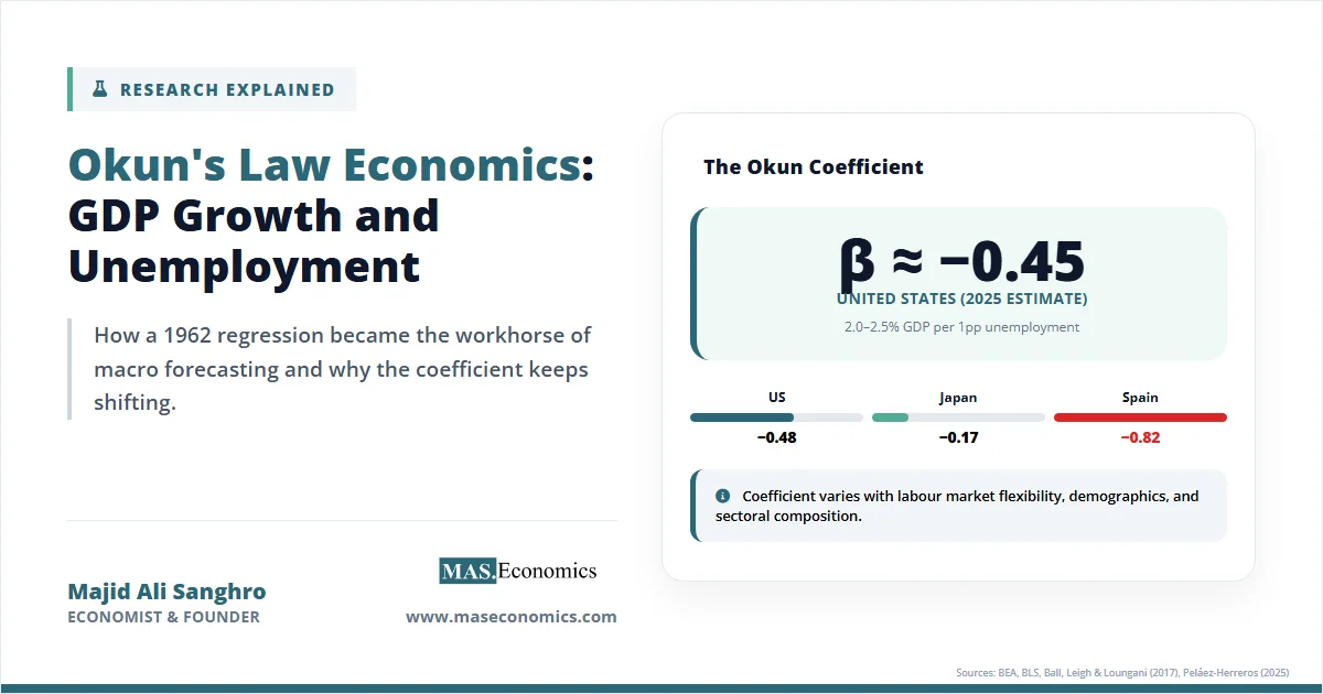
Six decades later, the relationship remains one of the most robust empirical regularities in macroeconomics. Ball, Leigh, and Loungani (2017) confirmed that the law holds across 20 OECD economies with annual data from 1980 to 2011, though with significant cross‑country variation in the coefficient. Modern estimates for the United States place the Okun coefficient at approximately –0.4 to –0.5 in the difference specification, smaller than Okun’s original three‑percent estimate.
Okun’s Law Formula and Equations
Okun’s Law economics rests on two complementary econometric specifications, each suited to different analytical purposes. The difference version operates directly on observable data and requires no estimate of unobservable potential output, making it the preferred workhorse for applied forecasting. The gap version is more theoretically grounded but depends on estimates of potential GDP and the natural rate of unemployment, both of which are subject to substantial measurement uncertainty.
The Difference Version
The difference version relates the change in the unemployment rate to the growth rate of real GDP:
Here, \( \Delta u_t \) represents the change in the unemployment rate from period \( t-1 \) to period \( t \), \( g_t \) is the annualised growth rate of real GDP in period \( t \), \( \alpha \) is the intercept (capturing the growth rate consistent with stable unemployment), \( \beta \) is the Okun coefficient, and \( \varepsilon_t \) is the error term. When real GDP grows faster than its trend rate (captured by \( -\alpha / \beta \)), unemployment falls; when GDP growth falls below trend, unemployment rises.
Okun’s original estimate yielded \( \beta \approx -0.3 \) on quarterly data from 1947 to 1960. Inverting this coefficient gives approximately 3.3, meaning that a one-percentage-point reduction in unemployment required roughly 3.3 percent additional GDP growth. Modern estimates using data through the 2020s typically yield \( \beta \) values between –0.4 and –0.5 for the United States, implying that the economy has become somewhat more responsive: each percentage-point change in unemployment now corresponds to roughly two percent of GDP rather than three.
The Gap Version
The gap version relates the unemployment gap to the output gap:
In this specification, \( u_t^* \) denotes the natural rate of unemployment (often approximated by the non-accelerating inflation rate of unemployment, or NAIRU), \( Y_t \) is actual real GDP, and \( Y_t^* \) is potential real GDP. The coefficient \( \beta \) measures the percentage-point change in unemployment associated with a one-percent deviation of output from its potential. For the United States, the inverted coefficient \( c = -1/\beta \) has historically ranged between 2 and 3, meaning that a one-percentage-point unemployment gap implies an output gap of roughly two to three percent of potential GDP.
The gap version is analytically richer because it directly connects to the concept of potential output and full-employment equilibrium. Its practical limitation is that neither \( u_t^* \) nor \( Y_t^* \) is directly observable. Estimates of potential GDP from the Congressional Budget Office (CBO), the OECD, or the IMF carry considerable uncertainty, particularly during periods of structural change. Measurement error in these trend variables can bias the Okun coefficient and inflate standard errors.
The Production-Function Decomposition
A deeper understanding of the Okun coefficient emerges from recognising that the relationship between output and unemployment is mediated by several labour market margins. Peláez-Herreros (2025) demonstrated that the Okun coefficient can be decomposed as follows:
The term \( \bar{e} \) represents the average employment rate (with a sign shift), and the \( \delta \) terms capture the indirect effects of changes in output per hour worked, hours per employed person, labour force participation, and working-age population growth. For the United States from 1970 to 2021, Peláez-Herreros estimated \( \beta = -0.475 \), composed of a direct employment-rate effect of –0.917 partially offset by positive indirect effects from productivity (0.076), hours adjustment (0.169), participation rate changes (0.149), and population growth (0.048).
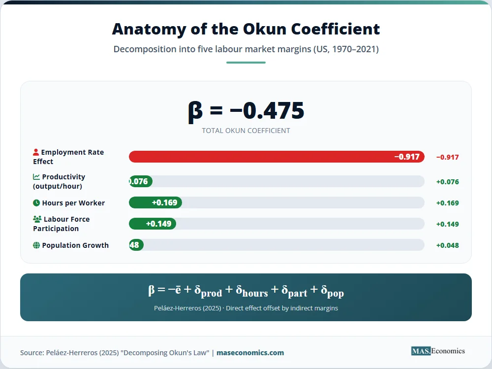
Table 1. Key Variables in Okun’s Law: Definitions and Notation
| Symbol | Variable | Description |
|---|---|---|
| \( \Delta u_t \) | Unemployment Change | Change in the unemployment rate between period \( t-1 \) and \( t \), measured in percentage points |
| \( g_t \) | Real GDP Growth | Annualised growth rate of real gross domestic product in period \( t \) |
| \( \beta \) | Okun Coefficient | The slope parameter measuring unemployment responsiveness to GDP growth; typically ranges from –0.3 to –0.5 for the United States |
| \( \alpha \) | Intercept | Captures the GDP growth rate consistent with a stable unemployment rate; reflects trend productivity and labour force growth |
| \( u_t^* \) | Natural Rate (NAIRU) | The unemployment rate consistent with stable inflation; unobservable, estimated via filtering or structural models |
| \( Y_t^* \) | Potential GDP | The level of output the economy can sustain at full employment without accelerating inflation |
| \( c = -1/\beta \) | Inverted Okun Coefficient | The percentage of GDP lost for every one-percentage-point increase in unemployment; typically 2 to 3 for the United States |

|
||
This decomposition clarifies why the Okun coefficient differs from unity. If output changes translated one-for-one into employment changes, and if every newly employed person came from the unemployment pool, then \( \beta \) would equal the negative of the employment rate (approximately –0.95 in the United States). The actual coefficient is roughly half that magnitude because firms absorb output fluctuations partly through hours adjustment and productivity variation rather than through hiring and firing alone.
Limitations of Okun’s Law
Okun’s Law is an empirical regularity, not a structural equation. Its stability depends on several implicit assumptions, and violations of these assumptions can cause the relationship to shift, flatten, or temporarily collapse.
The first assumption is linearity. The standard formulation posits a constant coefficient across the business cycle, yet a growing body of evidence suggests the relationship is asymmetric. Unemployment tends to rise more sharply during recessions than it falls during expansions of equivalent magnitude. Research covering 92 countries from 1980 to 2023 confirmed this pattern: the Okun coefficient is steeper during recessions, flatter during expansions, and statistically weaker or insignificant during recoveries, consistent with the phenomenon of jobless recoveries. Firms hoard labour during mild downturns but shed workers aggressively during deep recessions, while re-hiring during recoveries is constrained by uncertainty, retraining costs, and structural mismatch.
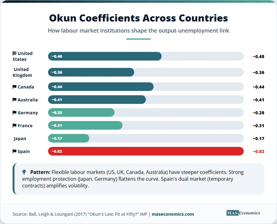
The second assumption concerns structural stability. The coefficient depends on the institutional architecture of the labour market: employment protection legislation, the prevalence of temporary contracts, unionisation rates, and the size of the informal sector. These features change slowly, which is why the law appears stable over medium-run samples. But over longer horizons or across countries, variation in these institutions produces substantial differences in the coefficient. Ball, Leigh, and Loungani (2017) estimated Okun coefficients of –0.17 for Japan, –0.48 for the United States, and –0.82 for Spain. Japan’s tradition of lifetime employment dampens the responsiveness of unemployment to output fluctuations, while Spain’s dual labour market, characterised by heavy reliance on temporary contracts, amplifies it.
The third assumption is that potential output and the natural rate of unemployment are stable or at least smoothly evolving. During periods of rapid structural change, such as the transition from manufacturing to services, the digital revolution, or the post-pandemic reshuffling of labour markets, estimates of potential output can shift abruptly. If potential GDP is overestimated, the gap version of Okun’s Law will understate the unemployment response to output movements, and vice versa.
A fourth and increasingly relevant limitation concerns the composition of employment. The gig economy, the expansion of part-time and contract work, and the rise of platform labour have blurred the boundary between employment and unemployment. Workers classified as employed may be substantially underemployed, and those classified as outside the labour force may be only marginally detached. These measurement issues introduce noise into the Okun relationship and may partially explain the weakening of the coefficient observed in some recent studies.
Finally, the COVID-19 recession of 2020 tested Okun’s Law in unprecedented fashion. GDP fell by approximately 31 percent (annualised) in the second quarter of 2020, while unemployment surged from 3.5 percent to 14.7 percent within two months. The subsequent recovery was equally anomalous: GDP rebounded by 33 percent in the third quarter, and unemployment fell rapidly as lockdowns eased and fiscal support sustained demand. These extreme observations lie far outside the historical range used to estimate the Okun coefficient, and including them in regression samples can destabilise estimates. Several studies have found that the COVID episode, while consistent with the directional prediction of Okun’s Law, produced residuals far larger than any historical episode, confirming that the law functions best as a guide to normal business-cycle fluctuations rather than as a predictor of tail events.
Empirical Evidence for Okun’s Law
The empirical track record of Okun’s Law economics is remarkably strong for a relationship that lacks a formal structural derivation. Ball, Leigh, and Loungani (2017) tested the law using data from 20 advanced economies and found that the relationship held in all countries except Austria and Italy, where the fit was poor. Across the sample, estimated coefficients ranged from –0.17 (Japan) to –0.82 (Spain), with most falling between –0.25 and –0.55. The average coefficient was approximately –0.40.
For the United States specifically, the law has remained stable across multiple estimation windows. Okun’s original 1947–1960 estimate yielded a coefficient of approximately –0.3 in the difference specification. Extending the sample to 2011, Ball et al. obtained estimates of –0.4 to –0.5 using both quarterly and annual data. The difference from Okun’s original estimate is largely attributable to sample composition and the inclusion of lags: Okun used a contemporaneous specification, while modern estimates typically include one lagged quarter of GDP growth, which captures the delayed adjustment of employment to output and strengthens the estimated coefficient.
The chart below presents the empirical Okun relationship for the United States using representative quarterly data points spanning 1960 to 2025. Each point represents a quarterly observation, with real GDP growth (annualised) on the horizontal axis and the change in the unemployment rate on the vertical axis. The fitted line represents the estimated Okun’s Law regression, and the negative slope confirms the inverse relationship.
Source: U.S. Bureau of Economic Analysis (BEA), U.S. Bureau of Labor Statistics (BLS). Representative quarterly observations, 1960–2025. | maseconomics.com
Several patterns emerge from the data. First, the negative relationship is visually evident: quarters with strong GDP growth cluster in the lower-right quadrant (falling unemployment), while recessions cluster in the upper-left quadrant (rising unemployment). Second, the scatter reveals meaningful dispersion around the fitted line, reflecting the influence of the additional margins (hours, productivity, participation) discussed in the decomposition above. Third, the COVID-19 quarters of 2020 appear as extreme outliers, with unemployment changes and GDP growth rates far exceeding historical norms.
Cross-Country Evidence
The cross-country pattern of Okun coefficients reveals the imprint of institutional design on the output-unemployment nexus. The table below summarises estimated coefficients for selected economies.
Table 2. Estimated Okun Coefficients Across Selected Economies
| Country | Okun Coefficient (\( \beta \)) | Inverted Coefficient (\( c \)) | Key Labour Market Feature |
|---|---|---|---|
| United States | –0.48 | 2.1 | Flexible hire-and-fire; weak employment protection |
| United Kingdom | –0.36 | 2.8 | Moderate flexibility; strong services sector |
| Germany | –0.28 | 3.6 | Kurzarbeit (short-time work) schemes; strong employment protection |
| Japan | –0.17 | 5.9 | Lifetime employment norms; internal labour markets |
| Spain | –0.82 | 1.2 | Dual labour market; extensive temporary contracts |
| Canada | –0.44 | 2.3 | Flexible, similar to U.S.; stronger EI system |
| Australia | –0.41 | 2.4 | Flexible with enterprise bargaining system |
| France | –0.31 | 3.2 | Rigid dismissal protections; high structural unemployment |
|
|
|||
The pattern is striking. Countries with flexible labour markets (the United States, Canada, Australia) exhibit larger Okun coefficients in absolute value, meaning unemployment responds more sharply to output fluctuations. Countries with strong employment protection or labour hoarding traditions (Japan, Germany) exhibit smaller coefficients, as firms absorb output declines through hours reduction and productivity adjustment rather than layoffs. Spain is an outlier in the opposite direction: its large coefficient (–0.82) reflects a dual labour market where temporary workers are hired and fired at very high rates, amplifying the cyclical volatility of unemployment relative to output.
Germany's experience during the 2008–2009 Global Financial Crisis provides a vivid illustration. Despite a GDP contraction of approximately 5.6 percent in 2009, Germany's unemployment rate rose by only 0.2 percentage points, an apparent violation of Okun's Law that was entirely explained by the widespread use of Kurzarbeit (government-subsidised short-time work). Firms reduced hours rather than headcount, shifting the adjustment from the extensive margin (employment) to the intensive margin (hours per worker). The Okun coefficient captures only the extensive margin, which is why it appears low for Germany.
More recent evidence from a 2025 study covering 92 countries from 1980 to 2023 confirmed that high-income and OECD economies exhibit robust Okun relationships across business-cycle regimes, while many low-income economies display weak or statistically insignificant coefficients, largely due to informality and structural rigidities in labour markets. In economies where a substantial share of the workforce operates outside formal employment statistics, the standard unemployment rate is a poor proxy for labour market slack, and Okun's Law loses its empirical grip.
Why Okun's Law Matters for Policy
Despite its limitations, Okun's Law economics remains deeply embedded in the infrastructure of macroeconomic policymaking. Its influence operates through several channels, and its practical applications extend far beyond the original question of estimating potential GDP.
Central Bank Forecasting and the Phillips Curve Connection
Okun's Law serves as one leg of a triangular forecasting framework used by central banks worldwide. The second leg is the Phillips Curve, which links unemployment to inflation. Together, these two empirical relationships form the backbone of the "workhorse" New Keynesian model used for monetary policy analysis. A central bank that wants to forecast inflation first estimates the output gap (using potential GDP models), then applies Okun's Law to translate the output gap into a predicted unemployment path, and finally uses the Phillips Curve to project inflation given the unemployment forecast.
The Federal Reserve, the European Central Bank, and the Bank of England all employ variants of this framework in their quarterly projections. The Okun coefficient determines the "speed limit" of output growth: how fast can GDP grow before unemployment falls below the natural rate, triggering inflationary pressure? When the Federal Reserve raised interest rates aggressively in 2022 and 2023, its projections of the associated labour market softening depended critically on the assumed Okun coefficient. A steeper coefficient implied that rate increases would produce larger unemployment effects for a given output slowdown, while a flatter coefficient implied that substantial output contraction would be needed to achieve even modest unemployment increases.
The post-2022 experience provided an important test of this framework. Despite the most aggressive monetary tightening cycle in four decades, U.S. unemployment remained historically low, rising only from 3.4 percent in early 2023 to approximately 4.3 percent by early 2026, even as GDP growth decelerated. This relatively modest unemployment response to significant monetary tightening is consistent with a flatter Okun coefficient in the post-pandemic period, potentially reflecting structural changes in labour supply, immigration-driven workforce expansion, and sectoral reallocation.
Fiscal Policy and the Output Cost of Unemployment
For fiscal policy authorities, Okun's Law provides a direct estimate of the output cost of unemployment. If the inverted coefficient \( c \) equals 2, then each percentage point of unemployment above the natural rate represents a two-percent shortfall in GDP relative to potential. For the United States in 2026, with a GDP of approximately $29 trillion, a one-percentage-point unemployment gap implies an output loss of roughly $580 billion per year. This calculation is central to cost-benefit assessments of fiscal stimulus programmes, fiscal multiplier estimation, and the evaluation of automatic stabilisers.
Okun himself used this framework to argue for active demand management. His 1962 paper was written in the context of the Kennedy administration's debate over tax cuts: if unemployment was 1.5 percentage points above the natural rate, and the Okun coefficient implied a three-percent output gap per unemployment point, then the economy was operating roughly 4.5 percent below potential, an enormous waste of productive capacity that targeted fiscal expansion could recover. The logic remains identical in contemporary policy debates over countercyclical fiscal policies and the appropriate pace of fiscal-monetary coordination.
Why the Coefficient Drifts
The most important contemporary debate surrounding Okun's Law concerns the stability of the coefficient itself. Several structural forces have been identified as potential drivers of long-run drift.
First, the shift from goods-producing to service-sector employment has implications for labour hoarding. Manufacturing firms face high fixed costs of hiring (training, capital-specific skills) and tend to hoard labour during downturns, producing a smaller Okun coefficient. Service-sector firms, particularly in hospitality, retail, and platform-based work, face lower adjustment costs and exhibit more volatile employment patterns, potentially steepening the coefficient. As the U.S. economy has shifted toward services, the Okun coefficient has increased in absolute value, consistent with this channel.
Second, labour market flexibility has increased in many OECD countries through deregulation, the erosion of collective bargaining, and the growth of non-standard employment. Greater flexibility means that firms can adjust headcount more rapidly in response to output fluctuations, which steepens the Okun coefficient. The rise of the gig economy and temporary staffing amplifies this effect.
Third, demographic shifts alter the coefficient through the participation-rate channel. An ageing population with a declining participation rate compresses the unemployment response to output fluctuations, because a larger share of the cyclical adjustment occurs through workers leaving the labour force entirely rather than becoming unemployed. This phenomenon was evident in the 2010s, when U.S. unemployment declined steadily even as GDP growth remained modest, partly because discouraged workers were exiting the labour force. The demographic transition across advanced economies may be gradually flattening the Okun coefficient by shifting adjustment from the unemployment margin to the participation margin.
Fourth, the rise of artificial intelligence and automation introduces a new dimension. If firms respond to cyclical downturns by accelerating automation rather than temporary layoffs, the recovery phase may feature "jobless" growth as output rebounds through productivity gains rather than re-hiring. This would flatten the Okun coefficient during expansions while potentially steepening it during contractions, reinforcing the asymmetry documented in the empirical literature.
Finally, the 2025–2026 tariff escalation and the broader trend of supply chain restructuring represent a potential structural break in the Okun relationship for trade-exposed economies. If tariff-induced reshoring creates new domestic manufacturing capacity, the resulting change in sectoral composition could alter the Okun coefficient by shifting employment toward industries with higher labour-hoarding tendencies. Conversely, if trade disruption leads to permanent job losses in export-oriented sectors, the coefficient may steepen temporarily as structural unemployment rises faster than output contracts.
Okun's Law in Developing Economies
The applicability of Okun's Law to developing and emerging economies is substantially weaker. In countries where the informal sector accounts for a large share of employment, such as India, Nigeria, or Indonesia, the official unemployment rate captures only a fraction of total labour market adjustment. Workers displaced from formal employment often transition into informal self-employment rather than registering as unemployed, muting the measured Okun coefficient. An ILO study found that for many developing countries, the coefficient was statistically insignificant or the wrong sign, not because the output-employment relationship was absent but because the unemployment rate was an inadequate summary of labour market conditions.
This limitation has practical consequences. Applying Okun's Law calibrated on U.S. or European data to forecast unemployment in developing economies is likely to produce misleading results. Policymakers in these contexts require alternative indicators, such as employment-to-population ratios, hours worked, or composite labour underutilisation measures, to capture the true relationship between output and labour market health.
MASEconomics Explains
4 economic concepts behind Okun's Law and the output-unemployment nexus
Conclusion
Okun's Law economics has endured for more than six decades as one of the most reliable empirical regularities in macroeconomics. The negative relationship between changes in the unemployment rate and real GDP growth, first documented by Arthur Okun in 1962 with U.S. data from 1947 to 1960, has been confirmed across dozens of countries and multiple estimation periods. Ball, Leigh, and Loungani (2017) demonstrated that the law fits data from 20 OECD economies with annual observations spanning 1980 to 2011.
The coefficient has evolved. Okun's original estimate of approximately –0.3 has been revised upward in absolute value to roughly –0.4 to –0.5 for the United States, reflecting changes in labour market structure, sectoral composition, and estimation methodology. Cross‑country variation in the coefficient, ranging from –0.17 for Japan to –0.82 for Spain, reflects the role of labour market institutions – employment protection, temporary contract prevalence, labour hoarding, and informal employment – in mediating the output‑unemployment nexus.
The coefficient is not constant. Structural forces, including the service‑sector transition, demographic ageing, the rise of platform labour, advances in artificial intelligence, and trade policy disruptions, can shift the Okun coefficient over time. The COVID‑19 pandemic demonstrated the law's limits in extreme tail events, while the post‑2022 experience of modest unemployment increases despite aggressive monetary tightening suggested a possible short‑run flattening of the relationship. The decomposition framework developed by Peláez‑Herreros (2025) clarifies that the coefficient is a reduced‑form summary of multiple adjustment margins; any structural change affecting productivity, hours, participation, or demographics will alter it.
The law's value lies in its robustness as a directional guide: when GDP grows above trend, unemployment falls; when GDP contracts, unemployment rises. The quantitative magnitude varies, but the qualitative relationship has survived every recession, recovery, and structural transformation of the past six decades.
Did you find this article helpful? Share it with someone who loves economics. And remember, at MASEconomics, we make complex ideas simple.