Stock markets and corporate boardrooms appear distant, but they share a fundamental linkage through the investment decisions of corporations. When stock prices soar, boardrooms approve new factories, research budgets, and equipment purchases. When markets crash, capital expenditure plans freeze. James Tobin, the Nobel laureate economist, provided the definitive theoretical bridge between these phenomena in 1969. Tobin’s Q Theory posits that the ratio of a firm’s market value to the replacement cost of its assets determines its incentive to invest. When the market values a firm at more than it costs to replace its physical capital, the firm should expand. When the market values the firm at less than its replacement cost, the firm should contract or liquidate. This single metric, the Q ratio, translates stock market fluctuations directly into real economic activity, making it a workhorse model for understanding corporate behaviour, monetary policy transmission, and the dynamics of the macroeconomy.
Before Tobin, the dominant theories of investment relied on interest rates and the marginal efficiency of capital, concepts heavily influenced by Keynesian cross and accelerator models. These frameworks, however, struggled to explain why firms with low borrowing costs sometimes refrained from investing, and why firms with high stock valuations aggressively expanded even when interest rates rose. Tobin reframed the problem by shifting the focus from the cost of borrowing to the price of capital relative to its replacement expense. By linking the financial market’s valuation of a firm to the real economy’s cost of building its assets, macroeconomic models gained a micro-founded mechanism for investment that remains central to modern analysis.
What Tobin’s Q Measures
The central insight of Tobin’s Q Theory is that a firm’s investment decision depends on the cost of acquiring capital from the stock market versus the cost of buying that capital in the goods market. The Q ratio is defined as the market value of a firm divided by the replacement cost of its assets. The market value is the total value of the firm’s outstanding equity and debt, representing what the financial market believes the firm’s future cash flows are worth. The replacement cost is the price the firm would have to pay to purchase all of its physical assets, such as factories, machinery, and inventory, at current market prices.
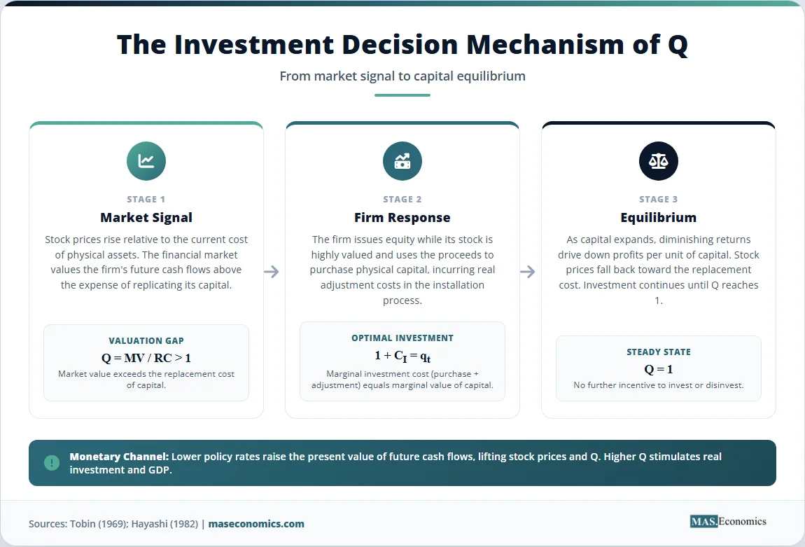
When Q is greater than one, the financial market values the firm’s assets at more than it would cost to replicate them. The firm, in effect, receives a signal that its capital is highly profitable. To capture this value, the firm should issue shares, use the proceeds to buy new machinery, and expand its operations. The cost of building a new factory is lower than the market’s valuation of that factory, making the investment a positive net present value project. Conversely, when Q is less than one, the market values the firm’s assets at less than their replacement cost. The firm could buy its own shares on the open market, or acquire a competitor, for less than it would cost to build new capacity. In this scenario, the firm should disinvest, halt new projects, and potentially liquidate existing assets to return capital to shareholders.
Tobin distinguished between two types of Q. Average Q is the ratio of the total market value of the firm to the total replacement cost of its assets. This is the observable metric that investors and economists calculate using balance sheet and stock market data. Marginal Q is the ratio of the change in the firm’s market value resulting from a one-unit increase in investment to the marginal cost of that new capital. Marginal Q governs the actual investment decision at the margin. Under specific assumptions, including constant returns to scale and perfect competition, average Q equals marginal Q, allowing the easily observable average Q to serve as a sufficient statistic for the firm’s investment behaviour. This equivalence is a powerful simplification that gives the theory its empirical bite.
The theory also implies that the stock market is not merely a sideshow or a casino, as some early Keynesians argued. Instead, the stock market is a central processor of information about the future profitability of capital. When stock prices rise, the cause is either improved expectations of future profits or a lower discount rate, both of which increase the incentive to invest. Market efficiency ensures that these prices aggregate dispersed information across millions of investors, translating their collective wisdom into a single signal that guides the allocation of real resources. The stock market thus functions as the economy’s steering mechanism for capital accumulation.
Tobin’s Q Theory in Equations
The formalisation of Tobin’s Q Theory begins with the firm’s value maximisation problem. The firm chooses its investment path to maximise the present discounted value of current and future cash flows, subject to a production technology and an adjustment cost function. Let \( V_t \) denote the market value of the firm’s capital stock at time \( t \). The firm’s capital stock \( K_t \) evolves according to the standard accumulation equation:
where \( I_t \) is gross investment and \( \delta \) is the depreciation rate. The key friction that makes Q matter is the assumption of adjustment costs. Without adjustment costs, the firm would instantly adjust its capital stock to the desired level, and investment would be infinitely elastic with respect to the interest rate. To generate a smooth investment path, the model assumes that installing new capital is costly. Let \( C(I_t, K_t) \) be the adjustment cost function, which is increasing and convex in investment: \( C_I > 0 \), \( C_{II} > 0 \). A common functional form is quadratic:
The firm’s problem is to maximise the present value of dividends, which are equal to operating profits minus investment and adjustment costs:
where \( F(K_t) \) is the firm’s operating profit as a function of its capital stock, satisfying the usual neoclassical conditions \( F_K > 0 \) and \( F_{KK} < 0 \). To solve this dynamic optimisation problem, we define the co-state variable \( q_t \) as the shadow price of an additional unit of capital, representing marginal Q. The Lagrangian for the firm’s discrete-time problem is:
The first-order condition with respect to investment \( I_t \) yields the optimality condition:
This equation states that the firm invests until the marginal cost of a unit of investment, including the adjustment cost, equals the marginal value of that capital, \( q_t \). Because the adjustment cost function is convex, a higher \( q_t \) implies a higher optimal level of investment. The relationship between \( q_t \) and investment is monotonically increasing, establishing the core prediction of the theory: investment is a positive function of marginal Q.
The co-state variable \( q_t \) evolves according to the Euler equation, which equates the return on capital to the market interest rate:
This condition shows that the value of capital today depends on its marginal product tomorrow, its remaining value after depreciation, and the effect of the larger capital stock on future adjustment costs. The transversality condition ensures that the present value of the shadow price converges to zero as time goes to infinity.
Fumio Hayashi (1982) proved that under the assumptions of constant returns to scale in production and adjustment costs, homogeneous capital, and perfect competition, marginal Q equals average Q. Average Q is defined as:
where \( V_t \) is the total market value of the firm, including debt and equity. Because average Q is observable from financial and accounting data, the Hayashi theorem allows empirical researchers to use \( Q_t^{avg} \) as a proxy for the unobserved marginal \( q_t \) in investment regressions. The table below summarises the key mathematical components.
| Variable | Definition | Role in the Model |
|---|---|---|
| \( Q_t \) | Tobin’s Q (marginal or average) | The key determinant of investment; high Q implies high investment |
| \( K_t \) | Capital stock at time t | Accumulates via investment and depreciates at rate \( \delta \) |
| \( I_t \) | Gross investment at time t | Chosen to maximise firm value subject to adjustment costs |
| \( C(I_t, K_t) \) | Adjustment cost function | Convex cost of installing new capital; ensures smooth investment |
| \( q_t \) | Shadow price of capital (marginal Q) | The co-state variable in the dynamic optimisation problem |
| \( V_t \) | Total market value of the firm | Numerator in the average Q calculation |
 | ||
Key variables in the mathematical formulation of Tobin’s Q Theory. The first-order condition \( 1 + C_I = q_t \) establishes the positive relationship between Q and investment.
Key Assumptions and Model Limitations
The elegance of Tobin’s Q Theory rests on several strong assumptions that, when violated, weaken the model’s predictive power and complicate its empirical application. Understanding these boundaries is necessary for interpreting the mixed empirical evidence the theory has generated over the past five decades.
The first and most famous assumption is the Hayashi (1982) condition that average Q equals marginal Q. This equivalence requires constant returns to scale in both the production function and the adjustment cost function, as well as perfect competition in product markets. If the firm has market power, as modelled in oligopoly or monopolistic competition, the marginal revenue product of capital is lower than the average product, causing average Q to overstate marginal Q. Similarly, if adjustment costs are not proportional to the firm’s size, the equivalence breaks down. In practice, firms have varying degrees of market power and face non-homogeneous adjustment frictions, meaning that average Q is an imperfect proxy for the marginal decision variable.
The second limitation is the assumption of perfect capital markets. The basic model assumes the firm can finance any positive NPV project, regardless of its internal cash flow or balance sheet structure. In reality, asymmetric information and agency costs create a wedge between the cost of internal and external finance, a friction formalised in the literature on capital structure. When external finance is costly, a firm with a high Q but low cash reserves may be unable to invest, while a firm with a lower Q but abundant cash flow may over-invest. This financial friction means that cash flow, not just Q, becomes a key determinant of investment, a finding confirmed by Fazzari, Hubbard, and Petersen (1988) and a vast subsequent literature.
Third, the model assumes homogeneous physical capital. In the modern economy, a large fraction of corporate value is derived from intangible assets, such as software, brand equity, research and development, and organisational capital. These assets are notoriously difficult to measure and are often excluded from the book value of capital used in Q calculations. When the denominator of the Q ratio omits intangibles, the calculated Q is artificially inflated, especially for technology and pharmaceutical firms. This measurement error biases the estimated relationship between Q and investment toward zero, making the theory appear less successful than it truly is. Peters and Taylor (2017) showed that correcting for intangible capital significantly improves the performance of Q in explaining corporate investment (Peters and Taylor, 2017).
Finally, the theory assumes that stock markets accurately reflect the fundamental value of the firm. If stock prices are driven by speculative bubbles, herd behaviour, or behavioural biases, then Q becomes a noisy signal of true investment profitability. A firm whose stock is overvalued may issue equity and invest the proceeds in low-return projects, simply because the cost of capital is temporarily depressed. This mechanism, sometimes called the “misvaluation channel,” complicates the welfare interpretation of the Q-investment relationship. High investment triggered by an inflated Q may lead to capital misallocation rather than genuine productivity growth.
Empirical Evidence for Tobin’s Q
The empirical performance of Tobin’s Q Theory has been the subject of intense debate since the first econometric tests in the late 1970s. The broad pattern in the data supports the theory’s qualitative prediction: firms with higher Q ratios do invest more. However, the quantitative relationship is weak. The coefficient on Q in investment regressions is typically positive and statistically significant, but the explanatory power of the model, measured by the R-squared, is low, and the estimated speed of adjustment is far slower than the theory predicts.
Early tests by von Furstenberg (1977) and Summers (1981) found that Q had a statistically significant effect on investment, but the coefficient was small, implying that firms responded very sluggishly to changes in market valuation. Furthermore, adding lagged investment or cash flow to the regression often swallowed the significance of Q, suggesting that financial frictions and adjustment dynamics not captured by the simple Q model were at work. The seminal paper by Fazzari, Hubbard, and Petersen (1988) showed that for firms that pay low dividends and are presumably financially constrained, cash flow is a powerful determinant of investment, while Q is relatively weak. For unconstrained firms, Q performs better, but even then, the model explains only a modest fraction of the variation in investment (Fazzari, Hubbard, and Petersen, 1988).
The chart below illustrates a stylised representation of the aggregate relationship between Tobin’s Q and gross private domestic investment as a share of GDP in the United States from 1990 to 2024. The series move together over the long run, confirming that high valuations are associated with high investment, but the correlation is far from perfect, especially during periods of market dislocation.
Stylised aggregate US Tobin’s Q ratio (left axis) versus Gross Private Domestic Investment as a share of GDP (right axis), 1990–2024. While the series share a broad upward trend during expansions, the correlation is noisy, reflecting financial frictions, measurement error, and the omission of intangible capital.
Recent research has revitalised the empirical case for Q by addressing the measurement error associated with intangible capital. Ryan Peters and Lucian Taylor constructed a measure of “Total Q” that incorporates the market value and replacement cost of intangible assets. Their analysis, published in the Journal of Financial Economics, found that Total Q explains a significantly larger fraction of corporate investment than traditional Q. When the denominator of the Q ratio is expanded to include knowledge capital, the estimated adjustment costs fall, and the relationship between market valuation and investment tightens considerably. This result implies that the poor empirical performance of Q in earlier decades was partly an artifact of mismeasurement, not a failure of the theory itself.
The table below contrasts the empirical predictions of the standard Q model with models that incorporate financial frictions and intangible capital.
| Empirical Dimension | Standard Q Model | Q Model with Financial Frictions | Q Model with Intangible Capital |
|---|---|---|---|
| Primary determinant of investment | Marginal Q | Q and internal cash flow | Total Q (including intangibles) |
| Effect of cash flow on investment | No effect (Modigliani-Miller holds) | Positive effect, especially for constrained firms | Smaller effect once intangibles are measured |
| Implied speed of capital adjustment | Slow (high adjustment costs) | Moderate | Fast (low adjustment costs for physical capital) |
| Performance for tech/R&D-heavy firms | Poor (Q is inflated) | Moderate | Strong (Total Q accounts for R&D stock) |
| |||
Comparison of standard, financially constrained, and intangible-adjusted Q models. The inclusion of intangible capital in Total Q significantly improves the empirical fit of the theory for modern corporations.
How Tobin’s Q Theory Shapes Investment Today
Tobin’s Q Theory remains an indispensable framework for understanding the intersection of financial markets and the real economy. Its applications span monetary policy, mergers and acquisitions, the economics of intangibles, and the analysis of corporate financial decisions. The model’s central insight, that the price of capital relative to its replacement cost drives real investment, provides a lens through which to interpret almost every major macroeconomic and corporate finance phenomenon.
The most important macroeconomic application is the monetary transmission mechanism. When a central bank lowers its policy rate, the discount rate applied to future corporate cash flows falls, raising the present value of those cash flows. Stock prices rise, and the Q ratio increases. This stimulates corporate investment, which in turn drives GDP growth. Conversely, when the central bank raises rates to fight inflation, stock valuations fall, Q declines, and investment contracts. This channel is a core part of the transmission mechanism in modern New Keynesian models, connecting directly to the IS-LM framework. The quantitative easing programmes implemented by the Federal Reserve, the European Central Bank, and the Bank of England after the 2008 financial crisis were explicitly designed to boost asset prices, raise Q, and stimulate investment. By purchasing long-term bonds and mortgage-backed securities, central banks pushed investors into riskier assets, including equities, propping up the Q ratio and supporting corporate capital expenditure (Bernanke, 2020).
In corporate finance and mergers and acquisitions, Q provides a clear theoretical prediction. When aggregate Q is high, firms should build new capacity. When aggregate Q is low, firms should buy existing capacity. This logic explains why M&A activity surges during bear markets and recessions. When the stock market values a target firm at less than the replacement cost of its assets, an acquirer can purchase those assets on the cheap through the stock market. The savings relative to building new factories or developing new products from scratch provide a powerful incentive to merge. The wave of distressed M&A during the 2008 financial crisis, and again during the early stages of the COVID-19 pandemic, is consistent with this mechanism. Firms with strong balance sheets and high Q ratios acquired distressed competitors with low Q ratios, consolidating assets at a discount.
The theory also provides a framework for understanding the rising share of share buybacks in corporate capital allocation. When a firm has a Q greater than one but lacks attractive physical investment opportunities or faces high adjustment costs, it may choose to return cash to shareholders. However, when Q is less than one, the firm should buy back its own stock. Repurchasing shares when Q is below unity is mathematically equivalent to buying capital at a discount, because the firm is acquiring its own assets for less than their replacement cost. The massive share buyback programmes executed by US corporations in recent decades are partly a reflection of this logic. Firms in mature industries with limited growth opportunities often have Q ratios close to or below one, making buybacks a value-maximising use of capital that signals confidence to the market.
The shift toward an intangible economy has made Q more relevant, not less, but only if the metric is measured correctly. For technology firms, pharmaceutical companies, and platform businesses, physical capital is a tiny fraction of total value. Traditional Q, calculated using only physical assets, generates astronomical ratios that imply implausibly large investment opportunities. The solution is not to discard Q, but to expand the denominator to include the firm’s stock of intangible capital, as proposed by Peters and Taylor. When research and development spending, software development costs, and brand investments are capitalised and depreciated, the Q ratio normalises, and its relationship to investment becomes robust. This adjustment is essential for applying the theory to the modern AI-driven economy, where the most productive capital resides in algorithms and data, not in blast furnaces and assembly lines. The discount rate used to evaluate these future cash flows ties directly into asset pricing models like the Capital Asset Pricing Model.
Furthermore, the theory sheds light on the phenomenon of secular stagnation. If the natural rate of interest falls, as proposed by Larry Summers and others, the steady-state Q ratio should rise, stimulating investment. However, if the underlying profitability of capital, the marginal product of capital, is declining due to a lack of innovation or demographic headwinds, then Q may remain depressed despite low interest rates. The relationship between the discount rate and expected cash flows in the Q formula explains why ultra-low interest rates in Japan and Europe did not generate the investment boom that standard monetary theory predicted. This demographic drag on the marginal product of capital is also a key component of the Solow-Swan growth model. The Q framework captures this nuance: it is not the interest rate alone that matters, but the ratio of the present value of cash flows to the replacement cost of capital.
MASEconomics Explains
Four economic concepts behind Tobin’s Q Theory
Conclusion
Tobin’s Q Theory provides the most robust theoretical link between financial market valuations and real corporate investment. By defining investment as a function of the ratio of market value to replacement cost, James Tobin showed that the stock market is not a mere casino but a vital processor of information that guides the allocation of physical capital. While early empirical tests found the model’s predictive power to be weak, subsequent research has shown that these failures were largely driven by the omission of intangible capital and the presence of financial frictions. When properly measured, Q remains a key determinant of corporate investment, mergers and acquisitions, and the monetary transmission mechanism. As the global economy continues to shift toward intangible assets, the framework requires careful measurement adjustments, but its core logic endures. As long as firms must decide whether to build new capacity or buy existing assets, the Q ratio will remain an indispensable tool for economists and investors alike.
Did you find this article helpful? Share it with someone who loves economics. And remember, at MASEconomics, we make complex ideas simple.