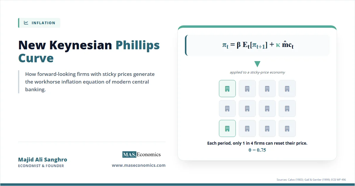
The new Keynesian Phillips curve replaces the original wage-unemployment relationship with a forward-looking equation linking current inflation to expected future inflation and real marginal cost. This framework emerged from explicit microfoundations, specifically monopolistically competitive firms facing Calvo-style staggered price-setting. The original Phillips curve, which posited a stable trade-off between inflation and unemployment, broke down empirically in the 1970s. The Lucas critique then showed that policy changes alter expectations, rendering historical relationships invalid. The New Keynesian response constructed a Phillips curve derived from optimising behaviour, ensuring policy invariance.
The Logic of Sticky‑Price Inflation
The original Phillips curve suggested policymakers could choose a permanent combination of inflation and unemployment. The stagflation of the 1970s destroyed that consensus. Simultaneously, the Lucas critique demonstrated that econometric policy evaluation must account for changes in private behaviour induced by policy itself. A new generation of economists sought to build a Phillips curve that could withstand these theoretical challenges by deriving aggregate inflation dynamics from first principles.
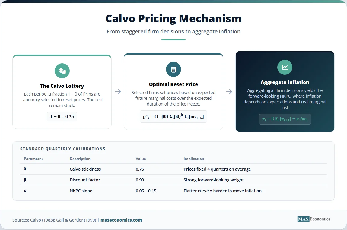
The New Keynesian approach begins with monopolistically competitive firms. Unlike firms in perfect competition, these firms set prices above marginal cost. However, they face a friction: they cannot adjust prices freely every period. Calvo (1983) introduced a probabilistic constraint where, in each period, only a fraction \( 1 – \theta \) of firms can reset their prices. The remaining fraction \( \theta \) must keep its prices unchanged. This staggered price-setting generates nominal rigidity at the aggregate level, even though individual firms desire continuous adjustment.
When a firm gets the rare opportunity to reset its price, it looks forward. It sets a price that maximises expected discounted profits over the entire duration the price might remain fixed. The optimal reset price depends on expected future marginal costs and expected future aggregate price levels. If a firm expects high marginal costs in the future, it sets a higher price today to protect its profit margins. Aggregating the decisions of resetting and non-resetting firms yields the structural inflation equation. Current inflation depends positively on expected future inflation and real marginal cost. There is no mechanical trade-off with unemployment. Any apparent short-run trade-off arises solely from nominal rigidities preventing immediate price adjustment. Inflation expectations become a primary driver of actual inflation, making central bank credibility the most important policy asset.
This theoretical structure resolved the failures of older Keynesian models. Because the relationship is derived from optimisation, it does not break down when the central bank changes its policy rule. Firms’ forward-looking behaviour ensures that any announced shift in monetary policy immediately alters pricing behaviour, consistent with the Lucas critique. The model also explained why disinflations often cause recessions: if the central bank lacks credibility, expected inflation adjusts slowly, and real marginal costs must bear the burden of reducing actual inflation, requiring contractions in economic activity.
NKPC in Equations
The mathematical derivation of the New Keynesian Phillips Curve begins with the Calvo pricing rule and builds to the aggregate inflation equation through log-linearisation around a zero-inflation steady state.
Calvo Pricing Rule
Each period, a fraction \( 1 – \theta \) of firms reset prices optimally. The parameter \( \theta \) measures price stickiness. The average price duration equals \( 1/(1-\theta) \) quarters. If \( \theta = 0.75 \), prices remain fixed for four quarters on average. This random selection mechanism implies that the probability of adjusting prices is independent of how long a firm has kept its price fixed, which is a simplifying assumption that makes the aggregation tractable.
Optimal Reset Price
A firm that can reset its price chooses \( p_t^* \) to maximise expected discounted profits:
Here, \( \beta \) is the household discount factor, reflecting the time value of money. The term \( mc_{t+k} \) is the log of nominal marginal cost, and \( p_{t+k} \) is the aggregate price level. The weight \( (\beta\theta)^k \) captures the probability that a price set today will still be in effect after \( k \) periods, which requires that the firm has not been drawn to reset in any of the intervening \( k \) periods. The reset price is a forward-looking weighted average of expected future nominal marginal costs. Higher stickiness \( \theta \) places more weight on the distant future, making current pricing decisions more dependent on long-run expectations.
Baseline New Keynesian Phillips Curve
Aggregating across firms yields the purely forward-looking NKPC:
where the slope parameter is:
The term \( \widehat{mc}_t \) represents real marginal cost in deviation from its steady state. When production is Cobb-Douglas with constant returns, real marginal cost equals the labour share of income. The parameter \( \kappa \) governs how strongly marginal cost pressures pass through to inflation. Higher price stickiness makes \( \kappa \) smaller, meaning marginal cost changes affect inflation slowly. A lower \( \kappa \) implies a flatter Phillips curve, requiring larger changes in real activity to move inflation.
Hybrid New Keynesian Phillips Curve
Galí and Gertler (1999) introduced a hybrid version allowing some firms to use backward-looking rule-of-thumb pricing. A fraction of firms, rather than optimising over the future, simply index their prices to past inflation. The hybrid specification is:
The parameters \( \gamma_b \) and \( \gamma_f \) are the backward-looking and forward-looking weights, respectively, constrained so that \( \gamma_b + \gamma_f \leq 1 \). This formulation captures intrinsic persistence in inflation, consistent with the empirical observation that inflation exhibits hump-shaped responses to shocks. Christiano, Eichenbaum, and Evans (2005) provided a microfoundation for indexation, showing that habit formation and wage stickiness can generate similar dynamics.
Output Gap Version
Substituting the relationship between marginal cost and the output gap \( \tilde{y}_t \), a common textbook reduced form emerges:
This version connects directly to the three-equation New Keynesian model, combining the NKPC with an IS curve and a monetary policy rule. The output gap formulation is analytically convenient but obscures the fact that the true structural driver is marginal cost, not the gap itself. Estimates of the slope \( \kappa \) can change significantly depending on whether the researcher uses the marginal cost or output gap specification.
Assumptions and Limitations
The NKPC relies on three core assumptions. First, the Calvo random price-resetting mechanism abstracts from realistic menu-cost models where firms choose when to pay a fixed cost to change prices. In reality, firms adjust prices strategically in response to large shocks, a feature captured by state-dependent pricing models (Dotsey, King, and Wolman 1999) but absent in Calvo time-dependent pricing. Second, rational expectations require that \( E_t \) represents model-consistent forecasts, meaning all agents understand the true structure of the economy. Third, constant elasticity of substitution demand from monopolistically competitive firms ensures a symmetric equilibrium where all resetting firms choose the same price.
Several key limitations emerge from these assumptions. First, the pure forward-looking NKPC predicts “jump” behaviour: inflation should respond immediately and fully to shocks. Empirical evidence, documented by Fuhrer and Moore (1995), shows hump-shaped inflation responses instead. Inflation rises gradually after a shock, peaks several quarters later, and then slowly reverts. The hybrid model addresses this by adding lagged inflation, but the backward-looking component is often viewed as an ad hoc fix rather than a deep structural feature. Without indexation, the baseline model generates counterfactual inflation dynamics.
Second, Generalised Method of Moments (GMM) estimates of \( \kappa \) are notoriously imprecise. Identification relies on finding valid instruments that correlate with marginal cost but not with the inflation error term. Weak instrument problems plague the empirical literature, making it difficult to reject both extreme price flexibility and extreme price stickiness. Mavroeidis (2005) demonstrated that standard NKPC specifications suffer from severe identification failures, meaning very different values of \( \kappa \) can fit the data equally well.
Third, the model assumes the output gap or real marginal cost is observable. Real marginal cost is unobserved and must be proxied, typically by the labour share. The output gap depends on estimates of potential output, which vary substantially across methodologies. Measurement choices materially change empirical results, creating a fundamental identification challenge for applied researchers.
Fourth, the baseline NKPC exhibits the “divine coincidence” identified by Blanchard and Galí (2007). Because the model lacks real wage rigidities, stabilising inflation automatically stabilises the output gap. In reality, policymakers face trade-offs between inflation and output stabilisation, particularly when supply shocks hit the economy. Adding real wage rigidities or cost-push shocks breaks the divine coincidence, but these additions reduce the model’s parsimony and complicate the policy implications.
Empirical Evidence for the NKPC
The empirical literature on the NKPC centres on estimating the relative weights of forward-looking and backward-looking behaviour. Galí and Gertler (1999) provided the foundational GMM estimation on US data spanning 1960–1997. Their innovation was using the labour share of income as the proxy for real marginal cost, rather than the output gap. Their results showed forward-looking dominance, with the forward-looking weight \( \gamma_f \approx 0.65 \) and the backward-looking weight \( \gamma_b \approx 0.35 \). This finding suggested that rational, forward-looking behaviour dominates inflation dynamics, even though intrinsic persistence exists. The labour share proxy, however, remains contested because its cyclical properties differ from traditional output gap measures.
Galí, Gertler, and López-Salido (2001) replicated this analysis for the euro area with similar results, finding forward-looking weights around 0.69. Their 2005 NBER working paper provided robustness checks responding to critiques from Rudd and Whelan (2005), reaffirming the forward-looking dominance using alternative estimators and specifications. They showed that the Rudd-Whelan results depended heavily on specific instrument choices and that broader instrument sets restored forward-looking dominance.
Rudd and Whelan (2005, JME) presented counter-evidence. Under their specification, lagged inflation matters substantially more than the Galí-Gertler framework suggests. They argued that the NKPC places too little weight on backward-looking behaviour to match the observed persistence of inflation. They also pointed out that real marginal cost, as measured by the labour share, has poor predictive power for future inflation, undermining the forward-looking narrative. This debate remains unresolved, with different identification strategies yielding different conclusions.
Rumler (2007), in ECB Working Paper 496, estimated open-economy NKPC models for nine euro area countries, finding average forward-looking weights around 0.62. Incorporating import prices improved the fit, showing that external supply shocks matter for domestic inflation dynamics in small open economies.
Microeconomic data provides a complementary perspective. The Atlanta Fed sticky-price CPI data shows that roughly 65% of consumer prices adjust less than once a quarter, consistent with the Calvo parameter values used in macro models. Nakamura and Steinsson (2008) found that the median price duration in the US is around 8–11 months for regular prices, though sales introduce substantial heterogeneity across sectors. Goods prices adjust more frequently than services prices, which helps explain why services inflation proves stickier during disinflationary periods.
Sources: BLS CPI; Bernanke and Blanchard (2024) decomposition framework.
| Symbol | Meaning | Typical Calibration | Source |
|---|---|---|---|
| \( \theta \) | Calvo price stickiness probability | 0.65–0.75 (quarterly) | Galí & Gertler (1999) |
| \( \beta \) | Household discount factor | 0.99 (quarterly) | Standard NK calibration |
| \( \kappa \) | Slope on real marginal cost | 0.05–0.15 | Galí & Gertler (1999) |
| \( \gamma_f \) | Forward-looking weight (hybrid) | 0.59–0.75 | Galí, Gertler, López-Salido (2005) |
| \( \gamma_b \) | Backward-looking weight (hybrid) | 0.25–0.41 | Galí, Gertler, López-Salido (2005) |
| Avg. price duration | Implied months between price changes | 9–12 months | Atlanta Fed sticky CPI |

|
|||
How the NKPC Matters
The New Keynesian Phillips Curve is the anchor of modern central bank Dynamic Stochastic General Equilibrium (DSGE) models. The Federal Reserve’s FRB/US model, the European Central Bank’s New Area-Wide Model, the Bank of England’s COMPASS, and the Bank of Canada’s ToTEM all embed a hybrid NKPC as their inflation block. These models serve as the primary quantitative tools for policy simulation and forecasting at the world’s leading monetary institutions. The conduct of monetary policy in advanced economies is inseparable from the NKPC framework.
In inflation forecasting practice, the NKPC is one of three pillars in the standard three-equation New Keynesian model. Alongside an IS curve describing output dynamics and a monetary policy rule describing interest rate setting, the NKPC determines the inflation path. Central bank staff produce forecast ranges by simulating this system under alternative shock scenarios. The framework’s structural nature allows policymakers to distinguish between temporary supply shocks and persistent demand pressures, informing the appropriate policy response.
The policy implication for forward guidance derives directly from the NKPC. Because expected future inflation enters the equation with weight \( \beta \approx 0.99 \), credible commitments about future policy rates feed directly into today’s inflation. If a central bank convincingly pledges to keep rates low for an extended period, firms and workers incorporate higher expected future inflation into their pricing and wage-setting decisions, raising current inflation without requiring any change in the current policy rate. This theoretical engine underpins the forward-guidance frameworks adopted by the Fed, ECB, and Bank of England following the 2008 financial crisis. However, the standard NKPC implies an excessively powerful forward guidance effect, known as the “forward guidance puzzle” (Del Negro, Giannoni, and Patterson 2015), where promises about rates in the distant future have implausibly large effects on current output and inflation. This puzzle has prompted modifications to the framework, including discounting of future expectations.
The 2021–2023 inflation surge tested the NKPC’s explanatory power. Whether the post-COVID surge reflects marginal-cost shocks from disrupted supply chains and energy prices or de-anchored expectations turns on which term in the NKPC dominates. Bernanke and Blanchard (2024) decomposed US inflation and found that supply-side shocks initially drove the surge, but tight labour markets and shifting expectations sustained it. This decomposition maps directly onto the NKPC structure: the \( \widehat{mc}_t \) term captures supply shocks, while the \( E_t[\pi_{t+1}] \) term captures expectation shifts. The analysis confirmed that both channels operate simultaneously, validating the hybrid NKPC’s dual emphasis on forward-looking expectations and current cost pressures.
The sticky-services inflation puzzle of 2024–2026 further validates the NKPC framework. Service prices adjust infrequently, consistent with high Calvo parameters. When services inflation proves resistant to monetary tightening, the NKPC predicts exactly this outcome: high \( \theta \) means a small \( \kappa \), so marginal cost reductions transmit slowly to services prices. The model explains why the last mile of disinflation requires maintaining restrictive policy longer than headline numbers suggest. Microeconomic data confirms that service prices change roughly half as frequently as goods prices, implying a flatter Phillips curve slope for the services sector.
Central banks in Australia, Canada, and the United Kingdom rely on hybrid NKPC specifications in their core policy models. The Reserve Bank of Australia’s MARTIN model, the Bank of Canada’s ToTEM, and the Bank of England’s COMPASS all estimate forward-looking and backward-looking weights similar to the Galí-Gertler findings. These calibrations inform interest rate decisions affecting millions of households. The flattening of the Phillips curve observed globally corresponds to a decline in the estimated slope \( \kappa \), making inflation less responsive to domestic output gaps and more responsive to global forces. This flattening complicates monetary policy because larger changes in the policy rate are required to move inflation by a given amount.
The theoretical structure also clarifies the causes of inflation. Cost-push shocks raise inflation through the marginal cost channel, while demand shocks raise inflation through the output gap channel. Expectation shocks shift inflation without any change in real economic activity. This three-way decomposition shapes how central banks diagnose inflation problems and design policy responses. Monetary transmission operates through the NKPC by influencing both the output gap and inflation expectations simultaneously. When a central bank raises interest rates, it contracts aggregate demand, reducing the output gap and marginal cost. It also signals commitment to price stability, anchoring expectations, and lowering the forward-looking component. The total effect on inflation combines both channels, which is why central bank communication is as important as the actual rate changes.
The NKPC also provides the intellectual foundation for inflation targeting regimes. If inflation depends on expected future inflation, then anchoring expectations at the target eliminates a major source of inflationary pressure. A credible central bank can achieve its inflation target with less output volatility than an unreliable one. This insight explains why central banks invest heavily in communication strategies, forward guidance, and transparency initiatives. The model demonstrates that reputation has real economic value: it reduces the sacrifice ratio, meaning less unemployment is needed to bring down inflation.
MASEconomics Explains
Four economic concepts behind the New Keynesian Phillips Curve
Conclusion
New Keynesian Phillips Curve theory has reshaped macroeconomic policy by replacing the discredited inflation-unemployment trade-off with a microfounded, forward-looking equation. Four facts stand out. First, the NKPC is derived from explicit microfoundations of optimising firms with staggered price-setting. Second, inflation is forward-looking: current inflation depends on expected future inflation, making expectations management the central task of monetary policy. Third, real marginal cost, not unemployment, is the structural driver of inflation pressure. Fourth, hybrid versions that allow backward-looking behaviour fit the data best, reflecting the empirical persistence of inflation. The NKPC remains the workhorse inflation equation inside the DSGE models used by major central banks worldwide, and it continues to frame debates about inflation diagnosis and policy design.
Did you find this article helpful? Share it with someone who loves economics. And remember, at MASEconomics, we make complex ideas simple.