Propensity Score Matching: Building Comparable Groups in Observational Studies

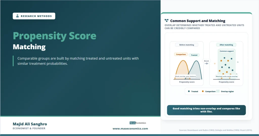
A job-training program, microcredit loan, health intervention, school scholarship, or firm subsidy often reaches people who are not randomly selected. Participants may be younger, poorer, more motivated, better informed, or closer to an implementing agency than nonparticipants. Propensity score matching is a research design tool that tries to construct a more credible comparison group by matching treated and untreated units with similar observed characteristics.

The method begins with a practical problem. In observational data, treated units and untreated units usually differ before treatment begins. A simple comparison of average outcomes may confuse the effect of treatment with pre-existing differences. If workers who join a training program already have different education, age, employment history, or motivation from workers who do not join, the raw outcome gap does not isolate the program effect.

Propensity score matching, often abbreviated as PSM, reduces this problem by summarizing many observed covariates into one score: the estimated probability of receiving treatment given pre-treatment characteristics. Treated and untreated units with similar scores are then compared. The method is powerful when selection is mostly captured by observed variables, but it cannot solve selection on unobserved factors. That boundary is the central lesson of PSM.

Propensity Score as a Covariate Summary

The propensity score was formalized by Paul Rosenbaum and Donald Rubin in “The Central Role of the Propensity Score in Observational Studies for Causal Effects”. Their key insight was simple but important: instead of matching treated and untreated units on every observed covariate directly, researchers can match on the probability of treatment conditional on those covariates.

Let \(D_i\) indicate whether unit \(i\) receives treatment, where \(D_i = 1\) for treated units and \(D_i = 0\) for untreated units. Let \(X_i\) represent observed pre-treatment characteristics. The propensity score is:

Propensity Score

The score is the probability of treatment given observed pre-treatment covariates.

In an economic application, \(X_i\) might include age, education, prior income, industry, location, household composition, baseline test scores, or firm size. A propensity score of 0.72 means the observed characteristics of that unit make treatment relatively likely. A score of 0.18 means treatment is less likely for a unit with that covariate profile.

The score itself is usually estimated with a logit or probit model, though modern applications may use more flexible methods when appropriate. The central idea is not the specific prediction model. The central idea is balance: after matching, the treated and comparison groups should look similar on observed pre-treatment variables.

Matching as a Design Step

PSM should be understood as a research design step, not merely as a statistical adjustment. The researcher first estimates treatment probabilities using only variables measured before treatment. Then the researcher uses those scores to form a comparison group. Only after that design step should outcomes be compared.

This ordering matters. If outcome variables influence the matching process, the design becomes contaminated by the result it is supposed to estimate. A careful PSM workflow resembles the logic of pre-analysis planning: define the treatment, covariates, matching rule, balance checks, and outcome analysis before letting the final outcome drive specification choices.

Suppose an economist studies whether a training program raises later earnings. Treated workers are program participants. Untreated workers are nonparticipants. Before matching, participants may be younger, less educated, or more recently unemployed. The researcher estimates each worker’s probability of participating based on pre-treatment characteristics, then matches participants to nonparticipants with similar scores. The final earnings comparison is made within this matched sample.

This places PSM inside the broader toolkit of causal inference. The method does not create random assignment. It tries to make an observational comparison more credible by making treated and untreated units comparable on observed covariates.

Selection on Observables Assumption

The main identifying assumption behind propensity score matching is often called selection on observables, conditional independence, or unconfoundedness. In plain language, once the researcher controls for observed pre-treatment variables, treatment assignment should be as good as random.

Conditional Independence

Potential outcomes are independent of treatment assignment after conditioning on observed covariates.

This is a strong assumption. It says that after accounting for observed characteristics, there are no remaining unobserved factors that jointly influence treatment and outcomes. If motivation, ability, political connections, health status, managerial quality, or access to informal networks affects both treatment and outcomes but is not measured, matching may still be biased.

This is the clearest distinction between PSM and a randomized experiment. In a randomized trial, randomization balances both observed and unobserved characteristics in expectation. In PSM, balance is targeted only for observed variables. A matched comparison can look excellent on measured characteristics while still being wrong because of unmeasured selection.

That does not make PSM useless. Many economic settings contain rich baseline data. Administrative records, surveys, firm panels, school records, and labor-market histories can sometimes capture important selection factors. But the credibility of PSM depends on the quality and relevance of the observed covariates, not on the matching algorithm alone.

Overlap and Feasibility

The second major condition is overlap, also called common support. Treated and untreated units must have comparable propensity scores. If some treated units have scores so high that no untreated units resemble them, there is no credible comparison group for those treated units. If some untreated units have scores far outside the treated range, they also contribute little to the treatment comparison.

Overlap Condition

For each covariate profile, there must be some chance of treatment and some chance of non-treatment.

Overlap is not a technical detail. It determines what population the study can speak about. If a microcredit program serves only the poorest households and untreated households in the data are mostly middle-income, matching may have little usable common support. If a firm subsidy reaches only very large exporters, small untreated firms cannot serve as credible matches.

This is why PSM often changes the estimand. The analysis may no longer estimate an effect for all treated units. It may estimate an effect for treated units who can be matched to similar untreated units. That narrower population may still be useful, but it should be described clearly.

Common‑Support Chart

A common-support plot helps readers see whether treated and untreated units occupy the same propensity-score range. The chart below is stylized. It shows that before matching, treated units tend to have higher treatment probabilities than untreated units. After trimming and matching, the usable comparison region is the

The shaded middle area is the part of the data where treated and untreated units can plausibly be compared. The left and right tails are weaker for matching because one group dominates. If the treated group and the comparison group barely overlap, PSM cannot rescue the design.

Common‑Support Chart

A common mistake is to treat the propensity score model like an ordinary prediction problem. The goal is not to predict treatment status as accurately as possible. The goal is to balance observed covariates between treated and untreated groups after matching.

A model that predicts treatment too well may reveal poor overlap: treated and untreated units are too different to compare. A model with high classification accuracy does not automatically produce better causal evidence. What matters is whether baseline characteristics are similar after matching.

Researchers usually assess balance with standardized mean differences, variance ratios, and visual diagnostics. The central question is simple: after matching, do the treated and comparison groups look similar on the variables that made selection likely?

Table 1. Balance Before and After Propensity Score Matching

Pre-treatment variable	Before matching	After matching	Interpretation
Age	Large gap	Small gap	Matching improved comparability
Prior earnings	Large gap	Small gap	Baseline economic status is closer
Education	Moderate gap	Small gap	Selection on schooling is reduced
Prior employment	Large gap	Moderate gap	Some imbalance remains
Design conclusion	Raw comparison is not credible		Matched comparison is more credible, but not automatic proof
Source: Stylized balance table based on standard PSM diagnostics. Entries are illustrative, not real data.

This table is deliberately qualitative. In a full empirical paper, the balance table would report standardized differences before and after matching. The important point is that matching should be judged by what it does to observed comparability, not by whether the treatment prediction model looks impressive.

Matching Algorithms Compared

After estimating propensity scores, researchers must choose how to match. Nearest-neighbor matching pairs each treated unit with one or more untreated units with the closest score. Caliper matching accepts a match only if the scores are close enough. Kernel matching uses weighted averages of many comparison units, with more weight on closer scores. Stratification divides observations into propensity-score blocks and compares treated and untreated units within each block.

These rules differ in how they trade bias and variance. Strict matching improves similarity but may discard many treated observations. Looser matching keeps more data but may compare units that are not sufficiently alike. Weighting methods use more observations but require careful diagnostics.

Caliendo and Kopeinig’s practical guide to propensity score matching emphasizes that implementation involves many decisions: selecting covariates, estimating the score, choosing a matching algorithm, checking common support, assessing match quality, and testing sensitivity to hidden bias. These choices should be justified as part of the research design.

The method chosen should match the study’s data structure. A small dataset with limited overlap may need careful calipers and trimming. A larger administrative dataset may support richer matching or weighting. In either case, the matching rule is not a substitute for theory, institutional knowledge, and careful measurement.

Estimands in PSM

Many PSM studies focus on the average treatment effect on the treated, usually written as ATT. This asks: among units that received treatment, what was the average effect compared with what would have happened to those same units without treatment?

Average Treatment Effect on the Treated

The untreated potential outcome for treated units is estimated using matched comparison units.

PSM is often well suited to ATT because the researcher starts from treated units and searches for comparable untreated units. But if many treated units lack good matches, the estimated effect may apply only to a subset of treated units inside common support. That is a narrower object than the effect for all treated units.

Other estimands are possible, including the average treatment effect for the full population, but they require different weighting or matching structures and stronger support across both groups. A good empirical paper should state which effect is being estimated and which observations are used to estimate it.

Hidden Selection Limitation

The most important limitation of PSM is that it only balances observed variables. If a treatment group differs from the comparison group on unobserved traits that affect outcomes, matching can still produce a biased estimate.

Consider an entrepreneurship training program. Suppose participants and nonparticipants are matched on age, education, region, prior income, and business sector. If participants are also more motivated, better connected, or more confident, and those traits affect later business income, the matched comparison may still overstate the training effect. The matching design can reduce observable imbalance without eliminating hidden selection.

This limitation is why PSM should be compared with other policy evaluation methods. Randomized controlled trials address both observed and unobserved selection through random assignment. Natural experiments use policy rules, shocks, or institutional variation that may create more credible treatment variation. Regression discontinuity design, when published and verified in the inventory, belongs in that same comparison because it uses a cutoff rather than observed similarity alone.

Importance of Baseline Data

PSM is strongest when the dataset contains the variables that actually drove selection into treatment. In labor economics, prior earnings and employment histories are often more informative than one-time demographic variables. In education research, baseline achievement, prior school quality, and family background may be essential. In firm-level studies, pre-treatment productivity, size, industry, location, and export status often matter.

Good data collection therefore comes before credible matching. A large dataset is not enough if it lacks the variables that explain treatment assignment. A smaller dataset with strong pre-treatment information may be more useful than a massive dataset with weak covariates.

Timing also matters. Covariates used for matching should be measured before treatment. Variables affected by treatment should not be included in the propensity score because they are part of the causal pathway, not pre-treatment confounders. Matching on post-treatment variables can block part of the treatment effect and create misleading estimates.

PSM vs Regression Adjustment

PSM and regression are often discussed together because both use observed covariates. But they work differently. A regression adjustment estimates the relationship between treatment, covariates, and outcomes in one model. PSM first constructs a more comparable sample, then compares outcomes within that matched design.

This distinction is useful. Multiple regression may extrapolate when treated and untreated units occupy very different covariate ranges. PSM makes overlap more visible by showing which units can and cannot be compared. It can reveal that the data do not support the comparison the researcher wanted to make.

In practice, many studies combine matching and regression. After matching, researchers may estimate an outcome regression on the matched sample to adjust for remaining imbalance. That can improve precision, but it should not hide weak overlap or poor balance. The design still depends on whether the matched sample provides credible comparison units.

Applications of PSM

PSM appears in labor economics, development economics, health economics, education research, public finance, firm studies, and program evaluation. It is especially common when a program has already been implemented and random assignment is unavailable. Dehejia and Wahba’s work on propensity score matching for nonexperimental causal studies helped show how matching could be used to evaluate training programs when experimental and nonexperimental data were both available for comparison.

Researchers may use PSM to study whether training raises earnings, whether microcredit changes business outcomes, whether health insurance affects medical use, whether school programs affect achievement, whether firm subsidies raise investment, or whether export promotion helps firms enter foreign markets. In each case, the key question is not simply whether treated units did better. It is whether the matched untreated units represent a credible counterfactual.

PSM also has a role in research transparency. By forcing the researcher to show common support and balance, it makes the comparison problem visible. That is valuable even when the final conclusion is that the data do not support a credible matched estimate. A method that reveals weak identification can still improve research quality.

Evaluating PSM Studies

A reader evaluating a PSM study should begin with the treatment assignment process. Why did some units receive treatment and others not? Are those reasons measured in the data? If important selection factors are missing, the design is weak even if the matching algorithm is sophisticated.

The second check is covariate timing. Matching variables should be measured before treatment. The third check is common support. Treated and untreated units should overlap across the propensity-score distribution. The fourth check is balance. After matching, observed characteristics should be similar across groups.

The fifth check is sensitivity. Does the result change when the matching rule, caliper, covariate set, or trimming rule changes? A result that survives reasonable design choices is more persuasive than one that appears only under a narrow specification. This links PSM to the broader problem of specification searching once that article is published and verified. Until then, the principle still applies: matching choices should be transparent rather than result-driven.

PSM vs Exact Matching

Exact matching pairs treated and untreated units with identical values on selected covariates. That can work when there are only a few covariates with limited categories. But in economic data, researchers often need to match on many variables. Exact matching can fail because very few units have identical covariate profiles.

The propensity score solves a dimensionality problem. It maps many covariates into one scalar probability. Treated and untreated units can then be compared by similar treatment probability rather than identical characteristics. Rosenbaum and Rubin showed that, under the relevant assumptions, balancing on the propensity score can balance the distribution of observed covariates.

This does not mean the score is magic. If the score is poorly estimated, if important covariates are missing, or if overlap is weak, the matched comparison remains questionable. The score is a tool for constructing a design, not proof that the design is valid.

Explains

Conclusion

Propensity score matching helps economists build comparison groups when treatment is not randomly assigned. It estimates each unit’s probability of receiving treatment based on observed pre-treatment characteristics, then compares treated and untreated units with similar scores. The method is most useful when it improves balance, reveals common support, and clarifies which units can credibly be compared.

Its strength is also its limit. PSM can reduce selection bias from observed variables, but it cannot remove bias from unobserved factors. A matched sample may look balanced on measured covariates while still being biased by motivation, ability, networks, expectations, or institutional access that the data do not capture. For that reason, PSM should be presented as a design for improving observational comparisons, not as a substitute for random assignment or a natural experiment.

A credible PSM study shows how treatment was assigned, why the covariates capture selection, where common support exists, whether balance improved, and how sensitive the estimate is to reasonable matching choices. When those pieces are transparent, propensity score matching can make observational evidence more disciplined. When they are missing, the matching algorithm may only give a weak comparison a more technical appearance.

Frequently Asked Questions

Thanks for reading! If you found this helpful, share it with friends and spread the knowledge. Happy learning with MASEconomics