Causal Diagrams DAGs: Mapping Assumptions in Research Design

A wage gap, school reform, health program, credit intervention, or tax change can look causal in a regression table while hiding the assumptions that make the estimate credible. Causal diagrams DAGs help researchers draw those assumptions before estimation by showing which variables cause which other variables, which paths create bias, and which controls may help or harm identification.

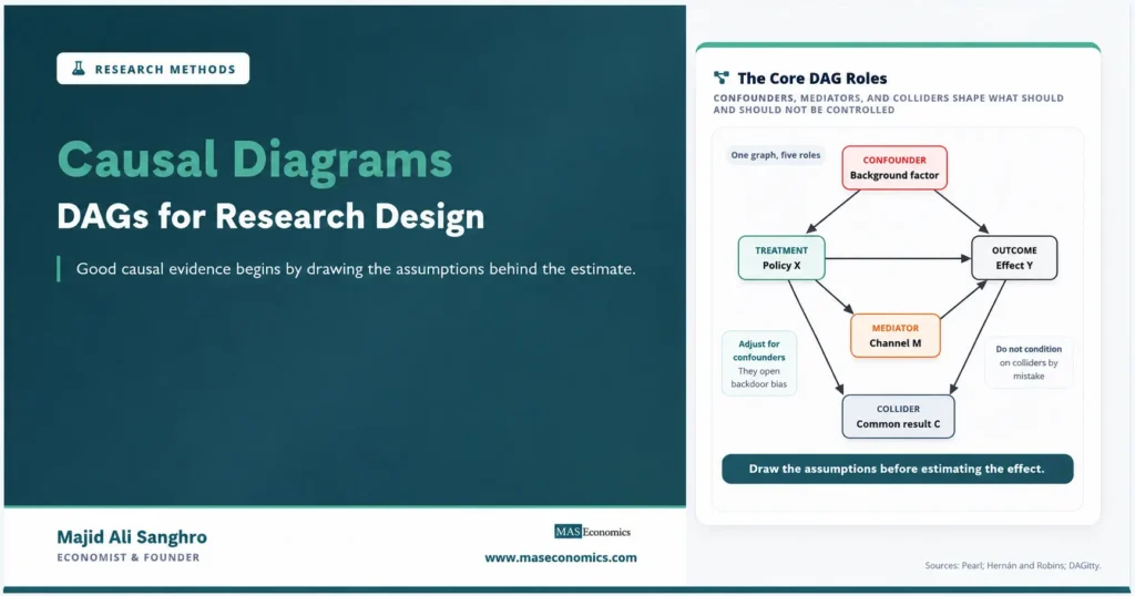
A directed acyclic graph, usually called a DAG, is a diagram made of nodes and arrows. The nodes represent variables. The arrows represent assumed causal directions. “Directed” means the arrows point from cause to effect. “Acyclic” means the arrows cannot loop back to the same variable. In research design, the purpose is not decoration. A DAG forces the researcher to state how treatment, outcome, confounders, mediators, colliders, and unobserved factors are believed to relate.

For economists, DAGs are useful because empirical questions rarely begin as clean equations. They begin as institutional stories: who gets treatment, who is exposed to a policy, who responds, who is measured, who is missing, and which variables are determined before or after treatment. A causal diagram turns that story into a visible structure. It does not prove that the assumptions are true, but it makes them explicit enough to evaluate.

DAGs Convert Stories to Designs

Every causal study needs a claim about what would have happened without treatment. In an experiment, random assignment helps justify that comparison. In observational research, the researcher must argue why treated and untreated units can be compared after accounting for selection, timing, institutions, and measurement. A DAG helps organize that argument.

Suppose an economist studies whether job training raises later earnings. Training is the treatment. Earnings are the outcome. Prior education, work experience, motivation, local labor demand, and program eligibility may affect both training participation and earnings. Some variables are observed. Others are not. A causal diagram asks the researcher to draw those relationships before deciding what to control for.

This makes DAGs part of causal inference, not a replacement for econometrics. The graph clarifies the assumptions behind the comparison. The estimator then uses data to estimate the effect under those assumptions. A regression, matching estimator, instrumental variable design, or discontinuity design can be technically correct and still answer the wrong question if the causal structure is misunderstood.

Judea Pearl’s Causality helped formalize graphical models as a language for causal assumptions. Hernán and Robins’ Causal Inference: What If shows how causal questions, counterfactuals, and diagrams fit into applied empirical work across disciplines. The common lesson is that causal claims require assumptions, and those assumptions should be visible before the estimates are interpreted.

Nodes and Arrows Convey Assumptions

A DAG starts with variables. A variable can be observed, such as income, education, age, or policy eligibility. It can also be unobserved, such as ability, motivation, managerial quality, or political influence. The arrows show assumed direct causal effects among those variables.

If education affects earnings, the diagram includes an arrow from education to earnings. If parental background affects both education and earnings, parental background points to both. If job training affects later employment and employment affects earnings, employment may sit on a causal pathway from training to earnings.

The absence of an arrow is also an assumption. If the diagram does not include an arrow from political connections to subsidy receipt, it is saying that political connections do not directly affect treatment in the model, or that the researcher has chosen not to represent that pathway. That choice may be defensible, but it should be recognized as a research-design claim.

Table 1. Core DAG Elements in Research Design

DAG element	Research-design meaning	Economic example	Why it matters
Treatment	The policy, program, exposure, or intervention	Job training, subsidy, scholarship, credit access	Defines the causal effect of interest
Outcome	The variable the treatment may change	Earnings, employment, investment, test scores	Determines what effect is being estimated
Confounder	A pre-treatment cause of both treatment and outcome	Education affects training and earnings	Creates bias if not handled
Mediator	A variable on the pathway from treatment to outcome	Training affects skills, skills affect earnings	Controls can block part of the effect
Collider	A variable caused by two other variables	Program completion affected by ability and training	Controlling can open a biased path
Unobserved factor	A variable not measured in the dataset	Motivation, informal networks, managerial quality	May limit identification even with controls
Source: MASEconomics editorial synthesis based on Pearl (2009), Hernán and Robins, and DAGitty documentation.

Confounding as Backdoor Path

The most common use of DAGs is to understand confounding. A confounder is a variable that affects both the treatment and the outcome before treatment occurs. In graph language, it opens a backdoor path from treatment to outcome.

Consider a study of whether vocational training raises earnings. Prior education may increase the probability of entering training and also increase later earnings. If the researcher compares trainees with nontrainees without accounting for education, part of the earnings difference may reflect education rather than training. The path runs from training back to education and then forward to earnings.

Confounding Logic

Here, \(X\) is treatment, \(Y\) is outcome, and \(Z\) is a confounder that causes both.

In many cases, conditioning on a measured confounder helps block the backdoor path. That is the logic behind including pre-treatment controls in regression, matching on baseline covariates, or stratifying by observable characteristics. But the DAG matters because it clarifies which variables are confounders and which are not.

This is directly connected to propensity score matching. Matching is credible only when observed pre-treatment covariates capture the main sources of selection. A DAG helps decide which covariates belong in the matching design and which variables should be excluded because they occur after treatment.

Bias from Certain Controls

Economists often learn that adding controls makes estimates more credible. DAGs show why that is not always true. Some controls block biasing paths. Others block the causal effect itself or open a path that was previously closed.

A mediator is one example. Suppose training raises skills and skills raise earnings. If the goal is the total effect of training on earnings, controlling for skills blocks part of the causal pathway. The estimate then no longer measures the total effect of training. It measures a more limited direct effect holding skills fixed.

Mediator Path

Controlling for \(M\) blocks part of the treatment effect when \(M\) lies between treatment and outcome.

A collider is even more dangerous. A collider is a variable caused by two other variables. Conditioning on a collider can create a statistical association between its causes even when none existed before. This is sometimes called collider bias or selection bias.

Collider Path

Conditioning on \(C\) can open an association between \(X\) and \(U\).

For example, suppose program completion is affected by both training assignment and motivation. If the researcher analyzes only people who completed the program, the sample may create a relationship between assignment and motivation. That selection can bias the estimated effect on earnings. The problem is not the lack of a control. The problem is controlling, selecting, or conditioning on the wrong variable.

Illustrative DAG Structures

The following stylized gallery shows three common DAG structures. The first graph shows confounding, where a pre-treatment variable affects both treatment and outcome. The second shows mediation, where the treatment affects an intermediate variable that affects the outcome. The third shows a collider, where conditioning on a common effect can introduce bias.

The gallery shows why “control for everything” is not a reliable research rule. A variable’s role depends on where it sits in the causal structure. The same observed variable can be useful in one design and harmful in another if the research question changes.

DAGs Guide Control Selection

Control-variable choice is one of the most common points where research design can go wrong. A researcher may include controls because they are available, because previous papers used them, or because they improve model fit. DAGs push the researcher to ask a more precise question: which variables must be conditioned on to identify the causal effect?

The backdoor criterion provides the intuition. To estimate the effect of treatment \(X\) on outcome \(Y\), the researcher must block noncausal backdoor paths from \(X\) to \(Y\) without blocking the causal path or opening a collider path. In practice, this means choosing controls based on pre-treatment causal structure rather than predictive convenience.

This matters for multiple regression. Regression can adjust for covariates, but it does not know which covariates are conceptually valid. The software will estimate a coefficient whether the controls are confounders, mediators, colliders, or post-treatment variables. The DAG provides the design logic that the regression table cannot supply.

It also matters for p-hacking. When researchers choose control sets after inspecting results, statistical significance can become a product of specification search. A pre-specified DAG reduces that flexibility by making the intended adjustment set visible before estimation.

DAGs Separate Total and Direct Effects

Many empirical disagreements arise because researchers are not estimating the same effect. A total effect includes all pathways from treatment to outcome. A direct effect excludes one or more mediating pathways. DAGs clarify this distinction before the model is estimated.

Suppose a scholarship increases college completion by improving enrollment, reducing financial stress, and allowing students to work fewer hours. If the researcher controls for enrollment intensity or working hours, the estimate may no longer represent the total effect of the scholarship. It may represent a controlled direct effect after holding part of the mechanism fixed.

That can be useful if the research question is about mechanisms. It is misleading if the policy question asks whether the scholarship as a whole improves completion. The appropriate controls depend on the estimand, not on a general preference for more variables.

This is why causal diagrams fit naturally with policy evaluation methods. Evaluation is not only about whether a coefficient is significant. It is about which effect the coefficient is supposed to represent and whether the design identifies that effect.

Acyclic Property in DAGs

The “acyclic” part of DAGs can seem restrictive to economists because many economic systems contain feedback. Income affects education, education affects income. Prices affect demand, demand affects future prices. Firms invest in productivity, productivity affects future investment. Macroeconomic variables often move together through dynamic systems.

A DAG handles this by ordering variables in time or by simplifying the causal question. If current income affects next year’s education spending, and education affects later income, the graph can represent the sequence with time-indexed variables. The key is that arrows do not loop back within the same time slice.

This makes timing central. A variable measured after treatment cannot be treated like a baseline confounder. A variable determined before treatment may be a valid control. A variable measured during treatment may be a mediator. A variable affected by both treatment and unobserved factors may be a collider.

For economic research, DAGs therefore push the researcher to write down the timeline. When was treatment assigned? When were covariates measured? When was the outcome observed? When could agents respond? Many identification errors begin as timing errors.

DAGs Clarify Sample Selection

Selection can occur before treatment, after treatment, or at the point of measurement. A study of wages may include only employed workers. A study of loan performance may include only approved borrowers. A study of training effects may include only program completers. A study of firm productivity may include only surviving firms.

These samples are not neutral. Employment, approval, completion, and survival can be affected by treatment, unobserved ability, demand shocks, or baseline characteristics. Conditioning on the selected sample may open paths that bias the estimate.

This is closely related to sample-selection methods such as the Heckman selection model, but the DAG perspective comes earlier. It asks whether the observed sample itself is part of the causal structure. If the outcome is observed only for selected units, the research design must explain how selection affects identification.

DAGs can also improve data collection. If the diagram shows that baseline health, prior earnings, household constraints, or firm size are likely confounders, those variables should be measured before treatment. A dataset that omits central confounders cannot be fixed by a cleaner diagram after the fact.

Randomization Simplifies DAGs

Random assignment is often described as the gold standard because it breaks the link between treatment assignment and pre-treatment causes of the outcome. In a DAG, randomization removes incoming arrows into treatment from confounders, at least in expectation. That makes treated and control groups comparable before treatment.

But randomization does not eliminate all design questions. Attrition can occur after assignment. Noncompliance can break the link between assignment and treatment received. Spillovers can connect treated and control units. Measurement error can affect outcomes. Mediators can complicate mechanism analysis.

A randomized study can therefore still benefit from a DAG. The diagram can show assignment, treatment take-up, outcome measurement, attrition, spillovers, and baseline covariates. It can clarify whether the estimate is an intention-to-treat effect, treatment-on-the-treated effect, direct effect, or total effect.

This is the same logic that applies to regression discontinuity design. The cutoff may create credible local variation, but the researcher still needs to understand manipulation, covariate balance, treatment take-up, and outcome measurement. A diagram can make those assumptions easier to inspect.

DAGs as Assumption Maps

A DAG can make a weak design look tidy if the assumptions are wrong. Drawing a graph does not prove that an omitted arrow is absent, that a variable is measured correctly, or that no unobserved confounder exists. The diagram is a claim about the world, not a fact about the dataset.

That limitation is important. A researcher can draw a DAG in which treatment is independent of all unobserved causes, but readers should ask why that is plausible. Institutional knowledge, prior literature, timing, measurement, and diagnostic checks still matter. A DAG is strongest when it is connected to the actual assignment process and data-generating context.

Tools such as DAGitty can help researchers draw and analyze causal diagrams, including adjustment sets and biasing paths. Textor and coauthors describe DAGitty as a tool for evaluating graphical causal models and identifying valid adjustment sets. The software is useful, but it cannot supply the substantive economics. The researcher must still justify the arrows.

DAGs in Economic Research

DAGs are useful at several points in the research process. At the proposal stage, they help convert a broad question into a causal structure. At the data stage, they show which variables need to be measured before treatment. At the analysis stage, they guide adjustment sets and warn against bad controls. At the writing stage, they make the identification argument clearer for readers.

They are especially useful when the research design involves observational data, complex selection, multiple mechanisms, or possible post-treatment controls. Studies of education, labor markets, firm subsidies, health insurance, credit access, migration, public programs, and policy eligibility often contain these features.

DAGs also support internal validity because they clarify whether the estimated contrast can be interpreted causally inside the study setting. They support external validity less directly, but still help by showing which mechanisms or selection processes may differ across populations.

The greatest benefit is discipline. A DAG requires the researcher to distinguish confounders from mediators, causes from proxies, selection from treatment, and timing from association. That discipline improves the research design even before any estimate is produced.

Evaluating DAGs in Papers

Readers should not accept a DAG simply because it looks clean. The first question is whether the treatment and outcome are clearly defined. The second is whether every arrow has a plausible economic reason. The third is whether important omitted variables could create unblocked backdoor paths.

The fourth question is timing. Are the controls measured before treatment? Are any post-treatment variables being controlled for? Are selection variables caused by treatment or unobserved factors? The fifth question is whether the adjustment set follows from the graph rather than from model-fit convenience.

The sixth question is whether alternative diagrams would lead to different conclusions. If a small change in the graph changes the required controls, the empirical result should be treated cautiously. A strong paper explains why its DAG is plausible, not merely what adjustment set it produces.

These questions link DAGs to the broader scientific method in economics. A good diagram is a transparent hypothesis about causal structure. It should be open to criticism, revision, and evidence, not protected as a final answer.

Explains

Conclusion

Causal diagrams DAGs improve research design by making causal assumptions visible before estimation begins. They show which variables are assumed to cause treatment, outcome, selection, or measurement. They help identify confounders, mediators, colliders, and selection pathways that ordinary regression tables often hide.

Their main value is not graphical elegance. It is disciplined thinking. A DAG helps the researcher decide which variables to control for, which variables not to control for, which data must be collected, and which causal effect is actually being estimated. That makes the method especially useful in observational economics, where treatment assignment is rarely random, and selection is often central.

DAGs do not prove causality by themselves. They clarify what must be true for a causal interpretation to hold. When the arrows are grounded in theory, institutions, timing, and evidence, causal diagrams can strengthen empirical research. When they are drawn casually, they only disguise weak assumptions in a clean picture.

Frequently Asked Questions

Thanks for reading! If you found this helpful, share it with friends and spread the knowledge. Happy learning with MASEconomics