What is Econometrics? A Comprehensive Introduction

In 2025, the global economy produced an estimated 181 zettabytes of data, according to the IDC Global DataSphere Forecast, and the volume continues to double roughly every three years. Central banks, treasuries, finance ministries, and international organisations sit atop this torrent of information. What is econometrics: the systematic method for converting raw observational data into testable, quantitative statements about economic behaviour. Without it, economic theory remains a collection of untested propositions. With it, policymakers obtain numerical estimates of the effects of interest‑rate changes, tax reforms, trade agreements, and labour‑market regulations before those policies are implemented.

The Question Every Economic Model Must Answer

Economics supplies qualitative propositions. A textbook might state that household consumption rises when disposable income rises, that imports fall when the exchange rate depreciates, or that inflation and unemployment share an inverse short‑run relationship. None of those statements specifies how large the effect is. The central bank needs to know whether a 25‑basis‑point increase cuts inflation by 0.1 percentage points or by 0.5 percentage points. The finance ministry needs to know what fraction of a transferred income is spent. These are quantitative questions, and they are the questions econometrics is built to answer.

The term itself was coined by Norwegian economist Ragnar Frisch, who founded the Econometric Society in December 1930. Frisch, together with Jan Tinbergen, received the first Nobel Memorial Prize in Economic Sciences in 1969 for “having developed and applied dynamic models for the analysis of economic processes.” Frisch intended econometrics to unify economic theory, mathematics, and statistical inference into a single quantitative discipline. That unification remains the working definition. An influential formulation by Samuelson, Koopmans, and Stone describes econometrics as “the quantitative analysis of actual economic phenomena based on the concurrent development of theory and observation, related by appropriate methods of inference.”

The discipline splits naturally into two branches. Theoretical econometrics investigates the statistical properties of estimators and tests, proving, for example, that an estimator is unbiased, consistent, or efficient under specified assumptions. Applied econometrics deploys those tools on real‑world data to estimate parameters, test hypotheses, build forecasts, and evaluate policies. The two branches feed each other: applied work uncovers data pathologies that theory must address. Theory supplies new procedures that are applied and then validated. This interplay has produced the modern econometric toolkit, which extends well beyond the linear regression model into time‑series analysis, panel‑data methods, limited‑dependent‑variable models, and causal‑inference frameworks.

Econometrics in One Equation

Every econometric investigation begins with a theoretical relationship and then writes it in a form that observed data can confront. The fundamental building block is the population regression function (PRF). Consider the simple case in which a dependent variable \( Y \) is hypothesised to depend on a single independent variable \( X \). The PRF expresses the conditional expectation of \( Y \) given \( X \):

Because real-world data never lie exactly on a straight line, the observed value of \( Y_i \) for any unit \( i \) is the sum of the systematic part and a random disturbance:

Here \( \beta_0 \) is the intercept, the expected value of \( Y \) when \( X = 0 \). \( \beta_1 \) is the slope parameter, measuring the change in the expected value of \( Y \) associated with a one-unit change in \( X \). The term \( \epsilon_i \) is the error term (or disturbance), which captures all factors other than \( X \) that influence \( Y_i \), including omitted variables, measurement error, functional-form misspecification, and unmodeled randomness.

The PRF is unknown in practice because the full population cannot be observed. The econometrician works instead with a sample of \( n \) observations and estimates the sample regression function (SRF):

where \( \hat{\beta}_0 \) and \( \hat{\beta}_1 \) are estimators computed from the sample. The residual \( \hat{\epsilon}_i = Y_i – \hat{Y}_i \) is the sample counterpart of the population error. The method of ordinary least squares (OLS) chooses \( \hat{\beta}_0 \) and \( \hat{\beta}_1 \) to minimise the sum of squared residuals. Under the Gauss-Markov assumptions, OLS yields the best linear unbiased estimator (BLUE) of the population parameters.

When a model includes \( k \) independent variables, the PRF generalises to the multiple regression form:

In matrix notation, which becomes essential for understanding estimators beyond OLS, this is written as \( \mathbf{y} = \mathbf{X}\mathbf{\beta} + \mathbf{\epsilon} \), where \( \mathbf{y} \) is an \( n \times 1 \) vector, \( \mathbf{X} \) is an \( n \times (k+1) \) matrix of regressors, and \( \mathbf{\beta} \) is a \( (k+1) \times 1 \) parameter vector.

The table below catalogues the notation that appears throughout the econometrics literature.

Table 1. Core Econometric Notation

Symbol	Definition
\( Y_i \)	Dependent (or outcome) variable for unit \( i \)
\( X_i, X_{ki} \)	Independent (or explanatory) variable(s)
\( \beta_0 \)	Intercept parameter
\( \beta_1, \dots, \beta_k \)	Slope coefficients
\( \epsilon_i \)	Population error term (disturbance)
\( \hat{\beta}_j \)	Estimated coefficient (sample counterpart of \( \beta_j \))
\( \hat{Y}_i \)	Fitted (predicted) value of \( Y_i \)
\( \hat{\epsilon}_i \)	Residual: \( Y_i – \hat{Y}_i \)
\( \mathbf{y}, \mathbf{X} \)	Vector and matrix representations of the data
\( \mathbf{\beta} \)	Parameter vector

Where Econometrics Sits in Modern Policy

The reach of econometrics extends across every major economic governance institution. The International Monetary Fund describes the objective of econometrics as converting qualitative statements into quantitative ones, replacing “consumption rises with income” with the precise estimate that “consumption expenditure increases by 95 cents for every one dollar increase in disposable income.” That conversion is not a pedagogical exercise. It is the analytic foundation of monetary policy, fiscal planning, and financial regulation.

Central banks operate large econometric models, including dynamic stochastic general equilibrium (DSGE) models, reduced‑form vector autoregressions (VARs), and semistructural models, to produce the forecasts that inform interest‑rate decisions. When the Federal Reserve’s Federal Open Market Committee assesses whether the current stance of policy is appropriate, the staff’s judgment draws on projections from a suite of econometric specifications. The Bank for International Settlements has noted that “structural econometrics … allowed for policy analysis and the study of counterfactuals,” making it possible to ask what would have happened had a different policy path been chosen.

Governments use econometric evidence to evaluate programmes. A labour ministry that raises the minimum wage wants to know, not guess, whether the change reduced employment among young workers. The econometric answer comes from causal‑inference techniques such as difference‑in‑differences, regression discontinuity, instrumental‑variable estimation, and synthetic control methods. These methods isolate the effect of the policy from the tangle of other economic forces operating simultaneously.

In the private sector, econometrics drives forecasting and risk management. Asset managers estimate conditional volatility with heteroscedasticity‑robust models. Banks stress‑test loan portfolios using econometric models that link default probabilities to macroeconomic scenarios. Consulting firms quantify the demand response to price changes, the elasticity, because a firm that sets price without knowing the elasticity is operating without a compass.

The World Bank employs econometrics to compare the effectiveness of development interventions. Randomised controlled trials, when feasible, provide the clearest evidence. Where randomisation is impossible, quasi‑experimental econometric designs fill the gap. A recent World Bank publication illustrated how event‑study and difference‑in‑differences methods are deployed to assess the impact of policy reforms on outcomes ranging from school enrolment to agricultural productivity.

Econometrics is also deeply embedded in the analytical infrastructure of emerging‑market central banks. The Reserve Bank of India maintains a suite of structural macroeconomic models for inflation forecasting. The State Bank of Pakistan runs vector autoregressions and error‑correction models to understand the transmission of monetary policy in a dollarised, import‑dependent economy. The Central Reserve Bank of Peru publishes an inflation report each quarter that leans on a semi‑structural model estimated with Bayesian techniques. In each of these institutions, the core question of how interest‑rate changes propagate to prices and output receives a quantitative, model‑based answer rather than a narrative one.

The demand for econometric skills continues to rise. The United States Bureau of Labor Statistics reported roughly 15,880 econometricians employed nationally as of May 2025, with projected growth over the 2024–2034 period reflecting the broader appetite for data‑driven decision‑making across government, finance, technology, and consulting. Econometrics now sits alongside machine learning and data science in the analytic toolkit of large organisations, though the disciplines differ in emphasis. Econometrics prioritises causal identification and parameter interpretability. Machine learning prioritises prediction from high‑dimensional data. At the academic frontier, the line between the two is blurring: causal machine‑learning methods such as Double Machine Learning and causal forests bring the two traditions together to estimate heterogeneous treatment effects with high‑dimensional controls, a topic covered in the MASEconomics article on Causal Machine Learning for Economists.

When Econometric Models Fall Short

The standard linear regression model rests on a set of assumptions. When those assumptions hold, OLS produces reliable estimates. When they fail, the estimates can be biased, inefficient, or both. Four departures from the classical conditions appear frequently in observational data.

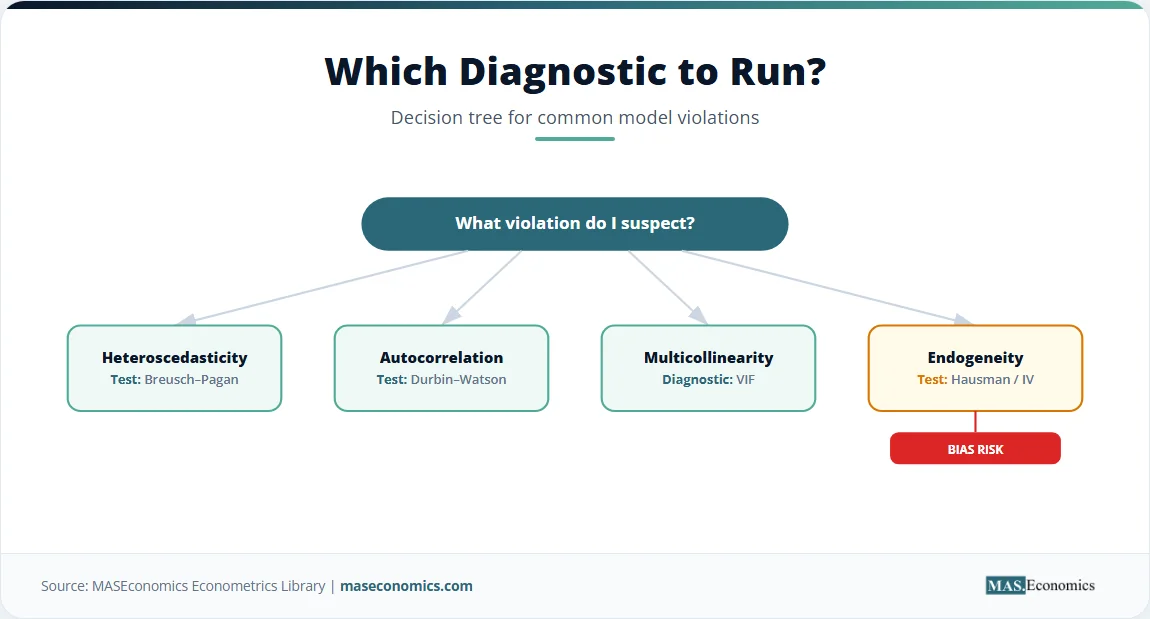
Multicollinearity. When two or more independent variables move together so closely that the data cannot distinguish their separate effects, coefficient estimates become imprecise. The variance inflation factor (VIF) quantifies the severity of the problem. The remedy, where feasible, is to collect more data, drop a redundant regressor, or use a shrinkage estimator. A detailed treatment of detection and correction appears in the MASEconomics article on multicollinearity.

Heteroscedasticity. If the variance of the error term is not constant across observations, the OLS estimator remains unbiased but is no longer efficient, and the standard formula for the standard errors is incorrect. Robust standard errors (White, or Huber–White) correct the inference. The article on heteroscedasticity walks through the Breusch–Pagan test and the robust‑covariance solution.

Autocorrelation. In time‑series data, errors from adjacent periods are often correlated. The Durbin–Watson statistic provides a first check. When autocorrelation is present, Newey–West standard errors restore valid inference. More advanced time‑series models, such as ARMA and ARIMA, along with their multivariate extensions, explicitly model the dependence structure rather than merely correcting for it. The autocorrelation article in the MASEconomics library covers detection and remedy in depth.

Endogeneity. The most consequential failure occurs when an explanatory variable is correlated with the error term. The cause may be an omitted variable that drives both \( X \) and \( Y \), simultaneity in which \( Y \) also causes \( X \), or measurement error in \( X \). Under endogeneity, OLS is biased and inconsistent, and no increase in sample size removes the bias. The solution requires an instrument, a variable correlated with \( X \) but uncorrelated with the error, and estimation via two‑stage least squares. The logic extends to the instrumental variables framework and, in its most general form, to the Generalised Method of Moments (GMM).

MASEconomics Explains

Conclusion

What is econometrics in summary: the empirical scaffolding that supports nearly every quantitative claim in modern economics. The discipline emerged from the insight, formalised by Frisch and the founders of the Econometric Society, that economic theory must be made to confront data through rigorous statistical inference. Its workhorse is the population regression function estimated by ordinary least squares, which remains the starting point for empirical investigation across macroeconomics, labour economics, finance, and development. Econometric models now sit inside the forecasting pipelines of every major central bank, inside the programme‑evaluation units of treasuries and international organisations, and inside the risk systems of financial institutions. The classical assumptions that guarantee OLS its desirable properties are routinely violated in observational data, and the field has produced a large catalogue of diagnostics and remedies to address each violation. Applied econometrics is therefore as much about testing and correcting the model as it is about estimating parameters.

The articles in the MASEconomics econometrics library, covering simple regression, multiple regression, time‑series analysis, panel data, and the diagnostic checks for heteroscedasticity, autocorrelation, and multicollinearity, build outward from the foundations laid here.

Thank you for reading! If you found this helpful, share it with friends and spread the knowledge. Happy learning with MASEconomics