The Slutsky equation answers a question that confused economists for nearly a century. When the price of a good falls, consumers buy more of it. But why? Are they buying more because the good is now relatively cheaper than its substitutes, or because their real purchasing power has risen, leaving them effectively wealthier? Eugen Slutsky, a Russian economist working in Kiev, published the answer in 1915 in an Italian journal called Giornale degli Economisti. His paper sat unread for two decades. When John Hicks and R.G.D. Allen rediscovered it in the 1930s, they recognised that Slutsky had solved one of the deepest problems in consumer theory: how to mathematically separate the two distinct forces hidden inside every price change.
That decomposition is the foundation of modern demand theory. It explains why central banks track substitution patterns when measuring inflation, why labour economists distinguish between wage effects on hours worked, and why public finance economists can separate the deadweight loss of a tax from its revenue effect. The equation is short. Its consequences run through almost every applied field in economics.
What the Slutsky Equation Does
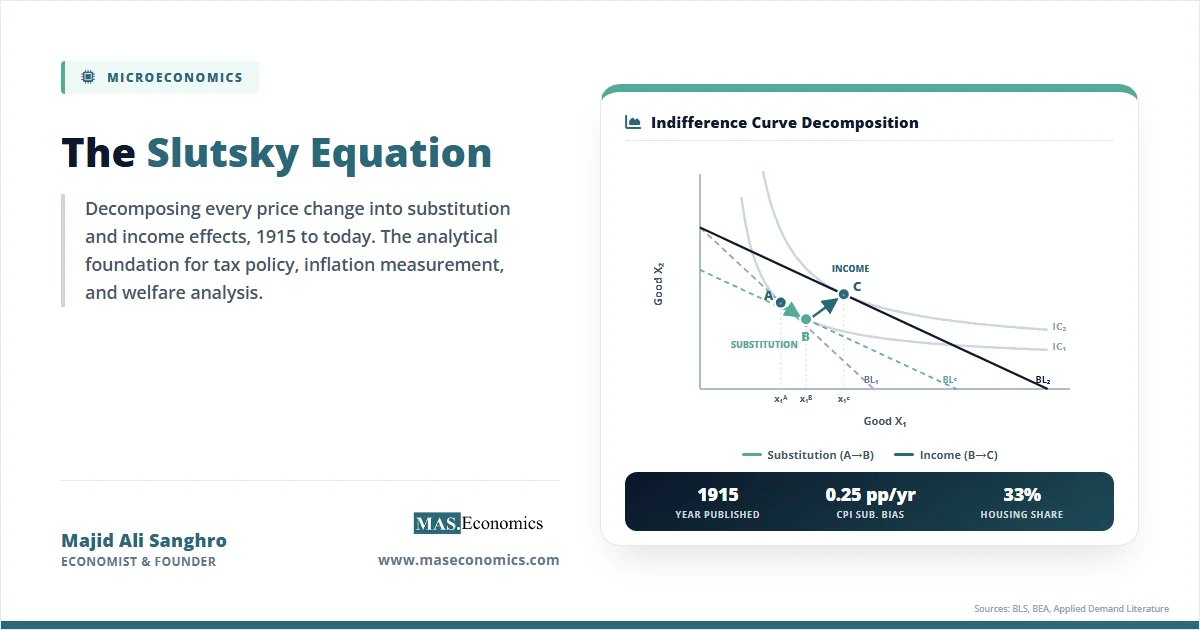
Consider a household that buys two goods: coffee and tea. The price of coffee drops by 20 percent. The household responds by buying more coffee. Standard demand analysis stops there, with the simple observation that quantity demanded rose because price fell. Slutsky asked a sharper question. The price drop did two things at once. It made coffee cheaper relative to tea, which would push the household toward coffee even if its overall budget were unchanged. It also made the household richer in real terms, because the original consumption bundle now costs less, freeing up money to spend on anything.
The first effect is the substitution effect. The second is the income effect. The total observed change in coffee consumption is the sum of these two forces. Slutsky’s contribution was to show that this decomposition is not just a useful intuition. It can be derived rigorously from the assumption that consumers maximise utility subject to a budget constraint, and the resulting equation has testable empirical content.
Before Slutsky, economists had vague verbal accounts of these forces. Alfred Marshall in his Principles of Economics distinguished income and substitution effects informally, but he treated the marginal utility of money as constant, which sidestepped the mathematical difficulties. Slutsky did not assume constant marginal utility. He worked directly with the demand functions implied by utility maximisation and derived the decomposition from the first-order conditions. The result was a partial differential equation linking observable demand responses to unobservable preferences.
The dilemma this solved was practical as well as theoretical. Demand curves slope downward almost always, but not invariably. Robert Giffen had reportedly observed that Irish potato consumption rose during the 1840s famine when potato prices climbed. Marshall mentioned this case in passing, and it became known as the Giffen good problem. Slutsky’s framework explained how it could happen. If a good is heavily inferior, meaning consumption falls as income rises, and it absorbs a large share of the budget, the negative income effect from a price increase can overwhelm the positive substitution effect away from substitutes. The demand curve then slopes upward. The mathematics made the conditions precise.
Slutsky Equation in Equations
Start with a consumer choosing quantities of two goods, \( x_1 \) and \( x_2 \), at prices \( p_1 \) and \( p_2 \), with income \( m \). The consumer maximises a utility function \( u(x_1, x_2) \) subject to the budget constraint \( p_1 x_1 + p_2 x_2 = m \). Solving this problem yields the Marshallian demand function, written as \( x_1^M(p_1, p_2, m) \), which gives the quantity demanded as a function of prices and income.
There is a second way to formulate consumer choice. Instead of maximising utility subject to a budget, the consumer can minimise expenditure subject to reaching a target utility level \( \bar{u} \). This dual problem yields the Hicksian demand function, written as \( x_1^H(p_1, p_2, \bar{u}) \). The Hicksian demand isolates the pure substitution response, because utility is held constant by construction. When prices change, the consumer is compensated with just enough income adjustment to stay on the original indifference curve.
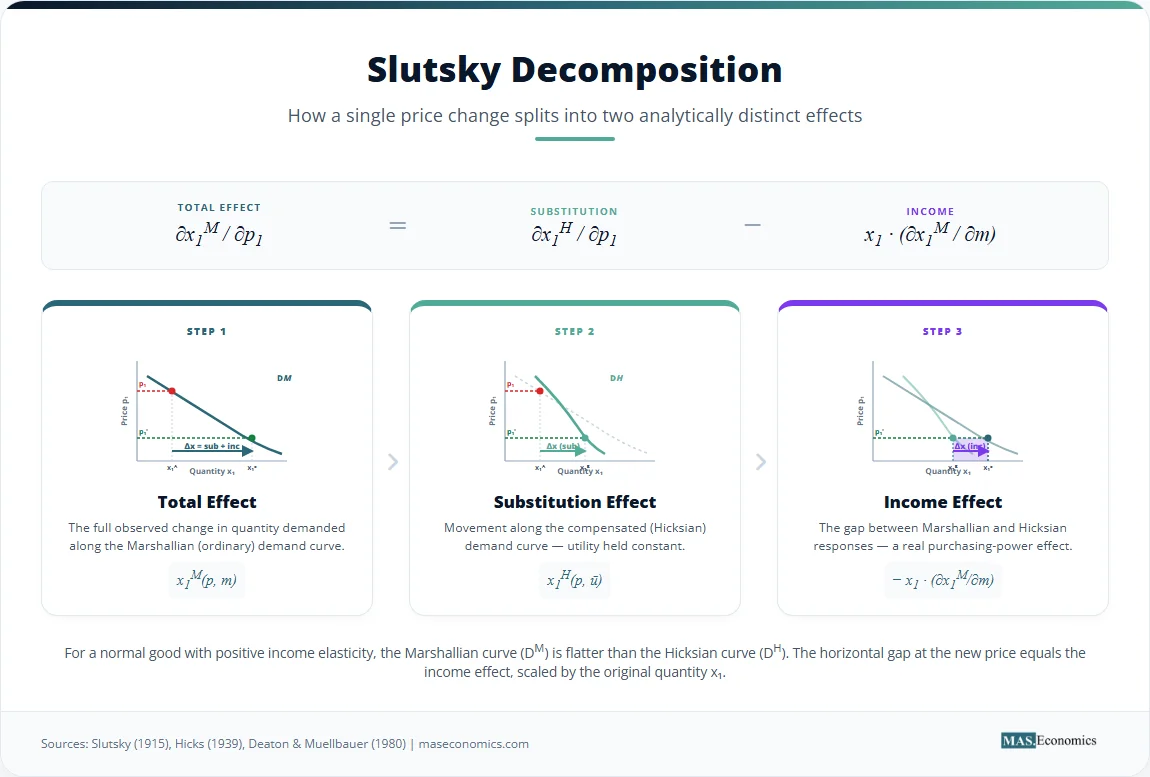
The Slutsky equation links these two demand functions. It states that the total derivative of Marshallian demand with respect to a price equals the Hicksian (compensated) derivative minus an income effect term:
The left side is the slope of the ordinary demand curve, the response economists actually observe in markets. The first term on the right is the substitution effect, which is always non-positive for the own-price case because of the curvature of indifference curves. The second term is the income effect, scaled by the quantity \( x_1 \) consumed, because a price change of one dollar on a unit of \( x_1 \) changes effective income by exactly \( x_1 \) dollars per unit of price change.
The derivation begins with the identity that Marshallian and Hicksian demands coincide at the optimum:
where \( e(p_1, p_2, \bar{u}) \) is the expenditure function, giving the minimum cost of reaching utility \( \bar{u} \). Differentiating both sides with respect to \( p_1 \) and applying the chain rule:
Shephard’s lemma gives \( \frac{\partial e}{\partial p_1} = x_1^H = x_1 \) at the optimum. Substituting and rearranging produces the Slutsky equation. The derivation is short, but its content is dense. It connects four different objects: the observable demand function, the unobservable compensated demand, the expenditure function, and the income response of demand.
The equation extends naturally to cross-price effects. The response of demand for good 1 to a change in the price of good 2 decomposes as:
This cross-price version is the basis for classifying goods as substitutes or complements. Two goods are net substitutes if the Hicksian cross-price derivative is positive, and net complements if it is negative. This classification depends only on the substitution term, not on income effects, which makes it a property of preferences rather than a property of the budget. The gross classification, based on the Marshallian derivative, conflates the two and can flip sign as income or budget shares change.
The substitution matrix, with entries \( s_{ij} = \frac{\partial x_i^H}{\partial p_j} \), has three properties that follow from utility maximisation. It is symmetric, so \( s_{ij} = s_{ji} \). It is negative semidefinite, which guarantees the law of demand for compensated changes. And it satisfies the homogeneity restriction that the row sums weighted by prices equal zero, reflecting the fact that proportional price changes with no income change leave compensated demand unchanged. These restrictions, often called the Slutsky symmetry and negativity conditions, are the central testable predictions of consumer theory.
| Symbol | Meaning | Interpretation |
|---|---|---|
| \( x_i^M \) | Marshallian demand for good \( i \) | Observed quantity at given prices and income |
| \( x_i^H \) | Hicksian demand for good \( i \) | Quantity at given prices, holding utility constant |
| \( p_i \) | Price of good \( i \) | Market price faced by the consumer |
| \( m \) | Money income | Total budget available to the consumer |
| \( \bar{u} \) | Target utility level | Reference well-being held constant in compensated demand |
| \( e(p, \bar{u}) \) | Expenditure function | Minimum cost of achieving utility \( \bar{u} \) at prices \( p \) |
| \( s_{ij} \) | Slutsky substitution term | Compensated cross-price response, \( \frac{\partial x_i^H}{\partial p_j} \) |
| \( \frac{\partial x_i^M}{\partial m} \) | Income effect on demand | Change in demand from a one-unit change in income |
 | ||
Variable reference for the Slutsky decomposition. The Marshallian and Hicksian demands differ only in what is held constant when prices change.
One more piece of notation is worth introducing. Multiplying through by \( p_1 / x_1 \) converts the equation into elasticity form:
Here \( \varepsilon_{11} \) is the Marshallian own-price elasticity, \( \varepsilon_{11}^H \) is the Hicksian own-price elasticity, \( s_1 = p_1 x_1 / m \) is the budget share of good 1, and \( \eta_1 = \frac{\partial x_1}{\partial m} \cdot \frac{m}{x_1} \) is the income elasticity. This form makes the empirical implications immediate. The wedge between observed and compensated price elasticity scales with budget share. For goods that absorb a tiny share of income, the income effect is small and Marshallian and Hicksian elasticities are close. For goods like housing or food that absorb large shares, the wedge can be substantial.
Assumptions Underlying the Slutsky Equation
The Slutsky equation rests on a small set of assumptions about the consumer. Preferences must be complete, transitive, and locally non-satiated, the standard axioms of rational choice theory. Demand functions must be differentiable, which rules out kinked preferences and fixed-proportion technologies at the level of analysis. The consumer must be a price taker, facing exogenous prices and choosing quantities. The budget constraint must hold with equality, which follows from local non-satiation but rules out savings and intertemporal choice in the static formulation.
None of these assumptions is innocuous. Behavioural economics has documented systematic violations of transitivity in laboratory and field settings. Prospect theory shows that consumers evaluate outcomes relative to reference points rather than over absolute wealth levels, which breaks the smooth utility function assumed by Slutsky. Satisficing models replace optimisation with rules of thumb, severing the link between observed choices and the underlying utility gradient.
The differentiability assumption hides another constraint. The equation as written applies to small price changes, treated as derivatives. Discrete changes require integration of the Slutsky terms, which in general depends on the path of integration unless the symmetry condition holds exactly. This is one reason symmetry tests are central to applied demand analysis. If the substitution matrix is not symmetric in the data, then no consistent utility function rationalises the observed behaviour, and welfare calculations based on the demand system are not well defined.
The static framework also assumes away dynamics. Habit formation, durable goods, and intertemporal substitution all require extensions. The Frisch demand function, which holds the marginal utility of wealth constant rather than utility itself, gives a cleaner decomposition for life-cycle problems. Permanent income models blend income and substitution effects across periods rather than across goods. The basic Slutsky logic survives in these settings, but the bookkeeping changes.
The equation comes in two distinct versions, and the difference matters. Slutsky’s original 1915 paper held real income constant in the sense of fixing the original consumption bundle. After a price change, the consumer is given enough income to afford the original bundle. This is the Slutsky compensation. Hicks, working with indifference curves, held utility constant instead, giving the consumer just enough income to reach the original indifference curve. This is the Hicks compensation. The two coincide for infinitesimal price changes but differ for discrete changes. Hicks compensation is theoretically cleaner because it ties directly to welfare, but Slutsky compensation is closer to what governments actually do when they index benefits to price changes through fixed consumption baskets.
Empirical Tests of the Slutsky Restrictions
The Slutsky restrictions provide sharp empirical predictions, and economists have tested them for decades. The results are mixed, instructive, and ongoing.
The earliest systematic tests came from Hendrik Houthakker and Lester Taylor in the 1960s, who estimated demand systems for major consumption categories using United States data. They found that homogeneity often held, but symmetry was rejected at conventional significance levels. Angus Deaton’s Almost Ideal Demand System, developed with John Muellbauer in 1980, became the workhorse for these tests. The AIDS framework allows direct estimation of the Slutsky restrictions, and applied work using consumer expenditure surveys from the United States, United Kingdom, Canada, and Australia has consistently shown that the symmetry condition is rejected for finely disaggregated goods, though the rejections weaken when goods are aggregated.
The pattern of rejections is itself informative. When researchers move from individual households to aggregated data, the symmetry conditions hold more easily, suggesting that aggregation across heterogeneous consumers smooths out individual deviations. When researchers focus on broad categories like food, housing, transport, and clothing, symmetry holds in most studies. When they zoom in on substitutes within a category, like different cuts of meat or different brands of cereal, the rejections multiply. Aviv Nevo’s 2001 study of the ready-to-eat cereal market found substantial asymmetries, which he attributed to brand-specific marketing and habit formation.
Field experiments have provided some of the cleanest tests. Natural experiments involving sudden price changes, such as the elimination of food subsidies or sudden tax reforms, allow direct estimation of price elasticities for specific populations. Robert Hutchens used welfare experiments in the 1970s to estimate Slutsky-decomposed labour supply responses, finding that substitution effects on hours worked were small but statistically present, while income effects were larger and dominated the gross response.
The income effect itself has been mapped extensively. U.S. Bureau of Labor Statistics data on consumer expenditures show that food, clothing, and housing all have income elasticities below one, making them necessities in the Engel sense. Restaurant meals, education, and recreation have elasticities above one, making them luxuries. These estimates feed directly into the Slutsky decomposition, allowing researchers to separate the two components for any observed price change.
The chart below shows the empirical relationship between budget share and the wedge between Marshallian and Hicksian own-price elasticities for major consumption categories in the United States, based on estimates synthesised from the Consumer Expenditure Survey and the Bureau of Economic Analysis. Goods with larger budget shares show larger gaps between observed and compensated elasticities, exactly as the Slutsky equation predicts.
Source: Author’s calculations using elasticity estimates from the Consumer Expenditure Survey, Bureau of Economic Analysis, and applied demand literature (Deaton and Muellbauer, Hausman, Nevo). The wedge measures the absolute difference between Marshallian and Hicksian own-price elasticities.
The pattern is clear. Housing, the largest budget item, shows the widest wedge between observed and compensated elasticities. Tobacco, with a tiny budget share, shows almost no wedge. The Slutsky decomposition predicts exactly this scaling, and the data confirm it across categories.
Giffen goods, the rare case where the income effect dominates, have proven difficult to identify in modern data. Robert Jensen and Nolan Miller’s 2008 study of rice and wheat consumption in Hunan and Gansu provinces of China found Giffen behaviour for very poor households where these staples absorbed over half of total expenditure. When the local government subsidised rice prices, consumption fell, exactly as the Slutsky framework predicts when a heavily inferior good with a large budget share gets cheaper. The income effect from cheaper rice freed up budget for meat and vegetables, and households shifted toward those goods even as rice became relatively cheaper. This study remains one of the few credible identifications of Giffen behaviour in field data, and its identification rested directly on the Slutsky decomposition logic.
The replication track record of demand system estimates is solid for aggregate categories and shakier for narrow ones, mirroring the pattern in applied microeconomics generally. The structural form of the Slutsky equation, however, is not in dispute. It is a mathematical consequence of utility maximisation, not an empirical hypothesis. What is tested is whether observed behaviour is consistent with utility maximisation at all, and the answer depends sensitively on aggregation, time horizon, and the specific goods studied.
How Slutsky Shapes Policy Today
The Slutsky decomposition is the engine behind most modern policy analysis that involves price changes. Tax policy, welfare measurement, inflation indexation, and labour supply estimation all rely on the ability to separate substitution from income effects, and the practical applications stretch from central bank statistics to court rulings on regulatory takings.

Consider the welfare cost of taxation. When a government imposes a tax on a good, the consumer faces a higher price and consumes less. The total reduction in consumption is the Marshallian response. But not all of this reduction represents lost welfare. Part of it reflects the income transfer to the government, which the government can in principle redistribute. The genuine deadweight loss is tied to the substitution effect alone, because that captures the distortion in choice that the tax creates beyond simply shifting purchasing power. Arnold Harberger’s classic deadweight loss formula, which underpins billions of dollars of tax policy analysis at the Congressional Budget Office and HM Treasury, is built directly from Hicksian demand curves. The Slutsky equation is what allows analysts to recover those Hicksian curves from observed Marshallian behaviour.
The deadweight loss formula, in its simplest form, is approximately:
where \( \tau \) is the tax rate. The key term is the Hicksian price derivative, not the Marshallian one. Without the Slutsky decomposition, applied analysts would either overstate or understate deadweight loss depending on whether the good has positive or negative income elasticity.
Inflation measurement is a second major application. The Consumer Price Index in the United States, the United Kingdom, Canada, and Australia is computed using a fixed basket of goods, which assumes consumers do not substitute when relative prices change. This Laspeyres approach systematically overstates the true cost of living because it ignores the substitution effect that the Slutsky equation isolates. The U.S. chained CPI, introduced by the Bureau of Labor Statistics in 2002, allows consumers to substitute and is therefore closer to a Hicksian cost-of-living index. The difference between the two indices, sometimes called substitution bias, has averaged 0.25 to 0.30 percentage points per year in U.S. data, which compounds to substantial differences over decades. Social Security cost-of-living adjustments have been debated for years on exactly this point, with reform proposals to switch to chained CPI explicitly motivated by the Slutsky logic.
Labour supply analysis is a third arena. When wages rise, workers face a higher price for leisure and a higher real income. The substitution effect pushes them to work more, since leisure is more expensive. The income effect pushes them to work less, since they can afford more leisure. The net response depends on the balance, which is exactly a Slutsky decomposition applied to the labour-leisure choice. Edward Prescott’s debate with Olivier Blanchard about why Europeans work fewer hours than Americans turned on this decomposition. Prescott argued that higher European tax rates explain almost all of the gap, working through the substitution effect on labour supply. Blanchard argued that preferences and institutions matter more, with smaller substitution effects than Prescott assumed. The empirical literature on labour supply elasticities, which informs tax policy in every developed country, is in essence a long argument about the size of the Hicksian compensated wage elasticity.
Public finance economists use the decomposition for optimal commodity taxation as well. The Ramsey rule, derived by Frank Ramsey in 1927 and refined by Peter Diamond and James Mirrlees in 1971, says that a revenue-maximising government should tax goods more heavily when they have small Hicksian elasticities. Goods with inelastic compensated demand can be taxed without much distortion. The intuition is direct: taxes distort by changing relative prices, and substitution effects measure how much consumers respond to relative price changes. Income effects, by contrast, are common to all goods and do not create allocative distortion. The Ramsey rule, every modern derivation of optimal tax theory, and the design of value-added tax systems in OECD countries all depend on this insight.
Antitrust analysis uses Slutsky symmetry to define markets. The U.S. Department of Justice and the European Commission both rely on diversion ratios, which measure how consumers shift between products when relative prices change. The compensated diversion ratio, which holds purchasing power constant, isolates pure substitution patterns and is the right measure for analysing whether two products compete in the same market. The 2010 Horizontal Merger Guidelines in the United States explicitly reference this approach, and the UPP (Upward Pricing Pressure) test used in merger reviews is derived from Slutsky-style decomposition.
Health economics applications include estimating the elasticity of demand for prescription drugs, hospital services, and health insurance. Jonathan Gruber’s research on health insurance subsidies in the United States separates the income effect of subsidies from the substitution effect across plan types, which matters for predicting how the Affordable Care Act would affect coverage decisions. The RAND Health Insurance Experiment of the 1970s and 1980s used random variation in insurance generosity to estimate compensated demand elasticities for healthcare services, and the resulting estimates have informed three decades of insurance design.
Energy economics offers another illustration. When fuel prices rise, households consume less fuel. Part of that response is substitution toward fuel-efficient vehicles and public transport. Part is the real income loss from a larger share of the budget going to fuel. Climate policy that prices carbon must distinguish these channels. The substitution response to a carbon tax is what generates emissions reductions. The income response, which is regressive because low-income households spend a larger share of their budget on energy, is what creates the political backlash. Carbon dividend proposals, which return tax revenue to households, are designed to neutralise the income effect while preserving the substitution effect, an explicit application of the Slutsky logic.
The equation also undergirds demand estimation in industrial organisation. When economists estimate residual demand curves for individual firms, they must control for income effects to identify the substitution patterns that determine markups and market power. The BLP demand model, developed by Berry, Levinsohn, and Pakes, builds the Slutsky decomposition into its discrete choice framework. Every recent merger case in the airline, telecommunications, and technology industries has involved BLP-style demand estimation, with the Slutsky restrictions providing identifying assumptions and welfare calculations.
Beyond these applied fields, the equation has shaped how economists think about welfare measurement itself. Compensating variation and equivalent variation, the two standard money-metric measures of utility change, are both derived from the expenditure function that sits behind the Slutsky equation. When the World Bank computes poverty thresholds in different countries, when the European Commission evaluates the welfare cost of trade barriers, and when the IMF estimates the impact of fuel subsidy reforms in developing economies, the underlying analytical framework traces directly to Slutsky’s 1915 derivation.
The equation has stayed relevant because it answers a question that does not go away. Every price change involves both a relative price effect and a real income effect, and any policy that involves prices, taxes, subsidies, or transfers must reckon with both. Slutsky gave economists a tool that converts an ambiguous behavioural response into two separately interpretable components. That tool is now built into the standard software packages used by central banks, finance ministries, and antitrust authorities across the developed world. It is also taught in every intermediate microeconomics course, where it serves as the bridge between graphical indifference curve analysis and the algebraic demand systems used in serious empirical work.
The reach of Slutsky’s framework extends to areas its author could not have anticipated. Behavioural welfare economics uses the decomposition as a benchmark against which to measure deviations from rational choice. Empirical industrial organisation builds models that nest the Slutsky restrictions as testable hypotheses. Even machine learning approaches to demand estimation typically impose Slutsky symmetry as a regularisation device, recognising that without some structure imposed by economic theory, flexible nonparametric estimators will overfit and produce nonsensical welfare predictions. A century after publication, the equation continues to discipline how economists translate observed behaviour into welfare conclusions.
MASEconomics Explains
Four economic concepts behind the Slutsky equation
Conclusion
The Slutsky equation remains the analytical core of consumer demand theory because it does something no other tool does: it converts an observable but ambiguous response into two separately interpretable components, each with its own welfare meaning and policy use. Substitution effects measure distortion. Income effects measure transfer. Tax policy, inflation measurement, labour supply analysis, antitrust enforcement, and welfare evaluation all rely on this distinction, and modern empirical work continues to test the symmetry and negativity restrictions the equation implies. The 1915 paper that introduced this framework was lost for two decades, but the equation it derived has organised consumer theory ever since. A century of empirical research has refined estimates of the two effects without overturning the underlying decomposition, and a century of policy work has applied the framework to questions Slutsky himself never imagined.
Did you find this article helpful? Share it with someone who loves economics. And remember, at MASEconomics, we make complex ideas simple.