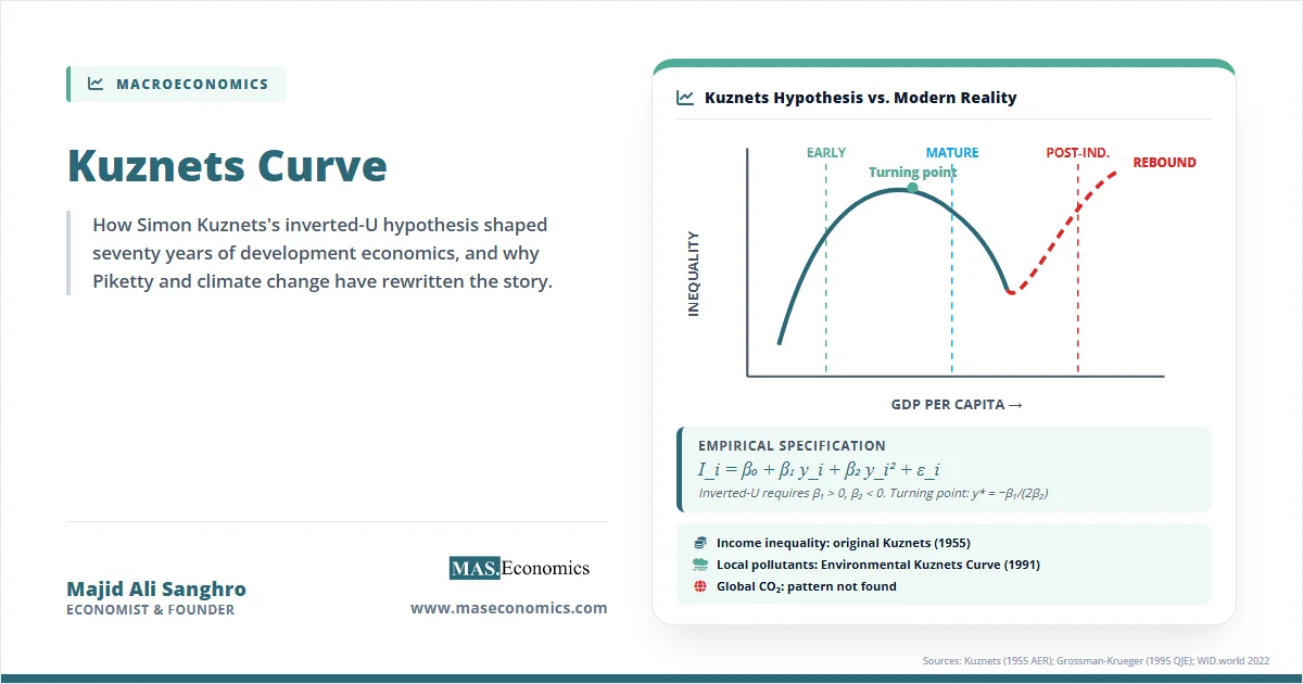
The Kuznets curve hypothesises that income inequality follows an inverted-U pattern as economies develop, rising in early industrialisation and falling as education and political institutions broaden. Simon Kuznets introduced this concept in his 1955 American Economic Review paper, observing the pattern in historical data for England, Germany, and the United States. The framework was later extended to environmental degradation through the Environmental Kuznets Curve, which applies the same inverted-U shape to pollution levels. However, 21st-century evidence from Piketty, Saez, and Zucman challenges the downward leg of the curve, showing that inequality has risen sharply in mature economies since 1980. The Solow-Swan growth model explains how economies expand, and endogenous growth theory shows how ideas drive that expansion, but the Kuznets curve attempts to explain who benefits from that growth.
What the Kuznets Curve Means
Simon Kuznets delivered his presidential address to the American Economic Association in December 1954, later published as “Economic Growth and Income Inequality” in 1955. Using limited historical data from three industrialised nations, Kuznets observed a striking pattern. During the early stages of industrialisation, income inequality widened as workers shifted from low-productivity agriculture to higher-productivity manufacturing. The owners of capital and the skilled factory workers pulled ahead of the rural population. However, as economies matured, inequality narrowed. Kuznets attributed this decline to the democratisation of education, the rise of labour unions, and the expansion of social welfare legislation.
The resulting graphical representation, plotting inequality against income per capita, resembles an inverted-U. Inequality rises during the early phases of growth, reaches a peak at middle-income levels, and then declines as countries achieve high-income status. This pattern became known as the Kuznets curve, and for decades it served as the dominant framework for understanding the relationship between economic development and income distribution.
In the early 1990s, economists Gene Grossman and Alan Krueger extended the logic to environmental quality. Their work, and that of Theodore Panayotou in 1993, proposed the Environmental Kuznets Curve. The hypothesis suggests that environmental degradation follows the same inverted-U trajectory: pollution intensifies during early industrialisation as economies prioritise output over environmental quality, but declines once countries reach sufficient income levels where citizens demand cleaner air and water. While intuitively appealing for local pollutants like sulphur dioxide and particulate matter, the Environmental Kuznets Curve has proven deeply controversial when applied to global externalities like carbon dioxide emissions.
Kuznets himself cautioned that his data were limited and his conclusions speculative. Modern evidence confirms this caution was warranted. The Acemoglu, Johnson, and Robinson research on institutions shows that political structures, not just sectoral shifts, determine inequality outcomes. And the long-run data compiled by Thomas Piketty and his colleagues demonstrate that the downward leg of the Kuznets curve reversed in most advanced economies after 1980.
Kuznets Curve in Equations
The Kuznets curve framework formalises the relationship between development and inequality through several key mathematical specifications, progressing from the measurement of inequality to the empirical models used to test the hypothesis.
Inequality Measurement: The Gini Coefficient
The most common summary measure of income inequality is the Gini coefficient:
where \(n\) is the population size, \(y_i\) is the income of individual \(i\), and \(\mu\) is the mean income. The Gini ranges from 0, representing perfect equality where everyone earns the same income, to 1, representing maximum inequality where a single individual receives all income. Most advanced economies have Gini coefficients between 0.25 and 0.45, while developing countries often exceed 0.50.
Kuznets Two-Sector Mechanism
Kuznets derived his hypothesis from a two-sector model where the population shifts from a low-mean, low-variance sector (agriculture, with share \(s\)) to a high-mean, high-variance sector (manufacturing, with share \(1-s\)). Total inequality decomposes into within-sector and between-sector components:
The between-sector component \(G_{\text{between}}(s)\) is a quadratic function of \(s\), maximised at intermediate transition stages when the population is split between the two sectors and falls to zero when \(s = 0\) or \(s = 1\). This mathematical structure generates the inverted-U pattern mechanically: as workers move from agriculture to manufacturing, the between-sector gap initially widens, pushing total inequality upward, then narrows as the agricultural share shrinks toward zero.
Empirical Kuznets Curve Specification
The standard empirical test of the Kuznets hypothesis regresses an inequality measure on income and its square:
where \(I_i\) is the inequality measure (typically the Gini coefficient), \(y_i\) is GDP per capita, and \(\mathbf{X}_i\) is a vector of control variables. The Kuznets hypothesis predicts \(\beta_1 > 0\) and \(\beta_2 < 0\), producing an inverted-U shape. The turning point, where inequality peaks, occurs at \(y^* = -\beta_1 / (2\beta_2)\). Early cross-country estimates placed this turning point between $5,000 and $10,000 per capita, though these estimates proved sensitive to specification and data quality.
Environmental Kuznets Curve Specification
The Environmental Kuznets Curve extends the framework to environmental degradation. A common specification adds a cubic term to capture potential N-shaped patterns:
where \(E_i\) represents environmental degradation (such as CO2, SO2, or particulate concentrations) and \(\mathbf{Z}_i\) includes relevant controls. The cubic term allows for the possibility that degradation initially rises, falls as environmental regulations take effect, and then rises again at very high income levels due to consumption-driven demand rebound.
Theil Index: An Alternative Decomposition
The Theil index offers an alternative inequality measure that decomposes cleanly into within-group and between-group components:
Bourguignon and Morrisson (2002) used the Theil index to construct global inequality estimates spanning 1820 to 1992, providing the longest available time series for testing Kuznets-curve dynamics at the world level. The decomposability of the Theil index makes it particularly useful for testing whether the between-sector mechanism Kuznets described actually drives the observed patterns.
Key Assumptions and Limitations
The Kuznets curve relies on three key assumptions. First, sectoral migration from agriculture to manufacturing is the dominant driver of inequality changes. Second, the within-sector inequality structure remains roughly stable over time. Third, institutions and politics evolve in tandem with development to redistribute income as societies become wealthier.
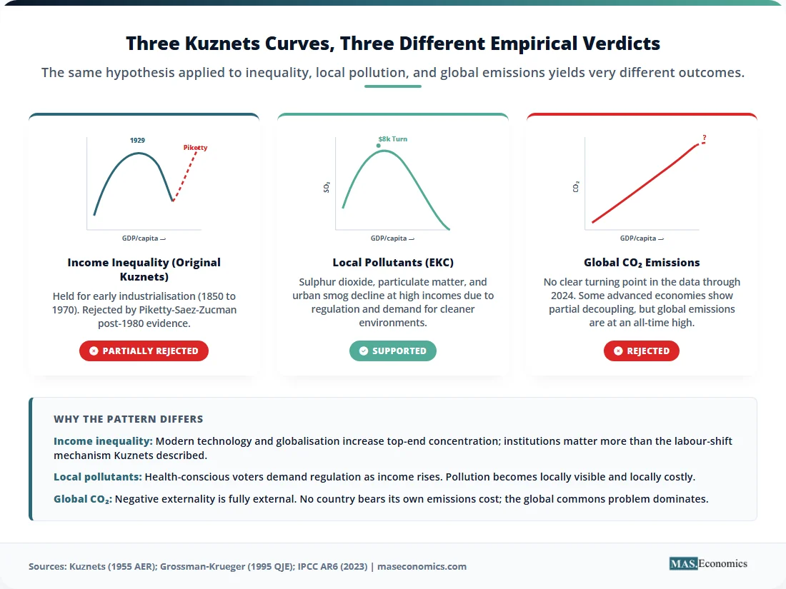
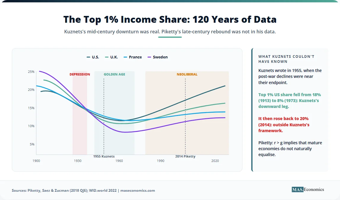
Several important limitations challenge these assumptions. First, Piketty (2014) demonstrated in “Capital in the Twenty-First Century” that inequality rose again in most rich economies after 1980. The rate of return on capital consistently exceeding the growth rate, expressed as \(r > g\), implies that wealth concentrates at the top unless disrupted by exogenous shocks like wars or deliberate policy interventions. The Kuznets downward leg is not a permanent feature of mature capitalism but a historical anomaly associated with the specific political conditions of the mid-20th century.
Second, Deininger and Squire (1996), using an improved cross-country panel dataset, found no robust inverted-U pattern once data quality and country-specific effects were properly accounted for. Their analysis showed that the apparent Kuznets curve in early studies was driven by a few outlier countries and cross-sectional variation rather than within-country dynamics over time.
Third, Kuznets’s original sample covered only three countries. This limited selection introduced sample-selection bias, as England, Germany, and the United States happened to experience declining inequality during the specific period he examined due to unique historical circumstances, including two world wars and the rise of redistributive welfare states.
Fourth, the Environmental Kuznets Curve works for some local pollutants but fails for CO2. Sulphur dioxide and particulate matter decline at high-income levels because citizens demand cleaner local air and governments respond with regulation. Carbon dioxide, as a global externality, does not trigger the same local demand for regulation, and global emissions continue to rise with income.
Fifth, the apparent turning point for pollution in some countries reflects the outsourcing of dirty industries to lower-income nations rather than genuine abatement. Stern (2004) documented this “globalisation reshuffle,” showing that the EKC for certain pollutants in rich countries is partly an artefact of shifting dirty production abroad.
Sixth, Acemoglu and Robinson (2002) argued that political institutions matter far more than the sectoral mechanism Kuznets described. Inequality declines when political coalitions empower workers and the middle classes, not automatically through sectoral reallocation. Without institutional change, development can perpetuate or even exacerbate inequality.
Empirical Evidence for the Kuznets Curve
The empirical literature on the Kuznets curve spans nearly seventy years and has undergone fundamental reversals. Kuznets (1955) based his hypothesis on historical national accounts from England, Germany, and the United States. His data showed inequality peaking around the late 19th or early 20th century and declining through the mid-20th century. This pattern appeared consistent across all three countries, lending initial credibility to the inverted-U hypothesis.
Bourguignon and Morrisson (2002), in a landmark American Economic Review paper, constructed global inequality estimates from 1820 to 1992 using the Theil index. Their data showed that global inequality between nations rose from the early 19th century to the mid‑20th century and has since stabilised, while within‑country inequality trajectories varied enormously. The global pattern was driven largely by the divergence between industrialising and non‑industrialising nations rather than by the within‑country mechanisms Kuznets described.
Deininger and Squire (1996) compiled a comprehensive panel dataset covering hundreds of country‑year observations. Their analysis rejected the universal Kuznets curve, finding that the inverted-U held for only a minority of countries in their sample. Most nations exhibited no statistically significant quadratic relationship between income and inequality. The results suggested that country‑specific institutions, policies, and historical conditions dominated any mechanical relationship between growth and distribution.
The Environmental Kuznets Curve received its first rigorous test from Grossman and Krueger (1995) in the Quarterly Journal of Economics. Using data from the Global Environmental Monitoring System, they found that sulphur dioxide and smoke (suspended particulate matter) concentrations followed an inverted-U pattern, peaking at around $8,000 per capita GDP. Panayotou (1993) formalised the EKC specification and estimated turning points for various pollutants. The EKC became influential in policy circles during the 1990s, with some commentators using it to argue that economic growth alone would eventually solve environmental problems.
However, the EKC does not hold for carbon dioxide emissions. Stern (2004) provided a comprehensive critique, showing that CO2 emissions per capita continue to rise with income even at the highest income levels. The IPCC Sixth Assessment Report (Synthesis Report, 2023) confirms that global greenhouse gas emissions continued to increase through 2019, with no clear turning point visible in the aggregate data. Our World in Data visualisations consistently show this divergence between local pollutant and global emission trajectories. Dasgupta, Laplante, Wang, and Wheeler (2002) confirmed in the Journal of Economic Perspectives that the environmental Kuznets curve has been flattening and shifting to the left, driven by economic liberalisation, clean technology diffusion, and new approaches to pollution regulation. Furthermore, current cross‑country Gini levels from the OECD Income Distribution Database show no universal decline in inequality among high‑income nations, further refuting the classic downward leg.
The most consequential challenge to the classic Kuznets curve comes from Piketty, Saez, and Zucman (2018), who constructed distributional national accounts for the United States. Their data showed that the top 1 percent income share fell from approximately 18 percent in 1913 to 8 percent in 1973, consistent with the Kuznets downward leg. But it then rebounded to 20 percent by 2014, far exceeding the earlier peak. The World Inequality Report 2022 extended this finding globally, showing that the post‑1980 increase in top income shares occurred in nearly all advanced economies.
Sources: World Inequality Database (WID.world); World Bank PovcalNet; OECD Income Distribution Database 2024.
| Version | Y-axis Variable | Predicted Pattern | Empirical Status (2025) | Key Source |
|---|---|---|---|---|
| Classic (Kuznets 1955) | Income inequality (Gini) | Inverted U with peak at mid-development | Mixed; rejected post-1980 by Piketty et al. | Kuznets (1955, AER) |
| EKC: Local pollutants | SO2, particulates, smog | Inverted U; turning point ~$8,000 GDP/cap | Supported (Grossman-Krueger 1995) | QJE 110(2) |
| EKC: Global pollutants | CO2 emissions per capita | Inverted U predicted | Rejected; emissions still rising | Stern (2004 WD); IPCC AR6 |
| N-shaped EKC | Various pollutants | U, upturn, second downturn | Found in some studies | Frontiers (2018) |
| Wealth Inequality (modern) | Top 1% wealth share | Should fall in mature economies | U-shaped rebound from 1980 | Piketty (2014); WID.world |

|
||||
How the Kuznets Curve Matters
The Kuznets curve framework has shaped how economists, policymakers, and international organisations think about development, inequality, and the environment for nearly seven decades.
First, the Kuznets curve defined the development economics paradigm for a generation. For decades, the inverted-U justified the view that developing countries would naturally see inequality rise and then fall as they grew. This logic influenced World Bank lending strategy and IMF stabilisation programmes from the 1960s through the 1990s. The implicit message was that short-term inequality increases were a necessary price for long-term convergence. If the Kuznets curve was correct, then the best way to reduce inequality was simply to grow the economy, and redistribution could wait until countries reached the turning point.
Second, Piketty’s challenge has fundamentally reframed the political economy of fiscal policy. The rise of what Piketty terms “patrimonial capitalism,” where \(r > g\) causes wealth to concentrate at the top, implies that mature economies cannot simply outgrow inequality. This insight has driven concrete policy changes. France’s digital services tax on large corporations, the global minimum corporate tax agreement under Pillar Two of the OECD and G20 BEPS framework establishing a 15 percent floor from 2024, and various wealth-tax proposals in the United States and Europe all trace their intellectual lineage to the Piketty critique of Kuznets. K-shaped recovery patterns following the COVID-19 pandemic further demonstrated that growth alone does not guarantee broadly shared prosperity.
Third, the Environmental Kuznets Curve played a significant role in climate policy debates. During the 1990s, the EKC was invoked in arguments against early action on emissions, with some claiming that economies would “grow their way out” of environmental problems. Subsequent evidence that CO2 does not follow the EKC pattern fundamentally changed the framing. The IPCC now explicitly rejects the idea that economic growth automatically reduces emissions, and the EU Emissions Trading System and the US Inflation Reduction Act of 2022 reflect the post-EKC consensus that deliberate policy intervention is necessary. Climate adaptation costs are now modelled as unavoidable investments rather than temporary burdens that growth will eliminate.
Fourth, the World Inequality Database, built on the Piketty-Saez-Zucman methodology, has become a standard tool for international organisations. The IMF uses WID data in Article IV consultations, the World Bank’s Poverty and Inequality Platform incorporates distributional national accounts, and the OECD Income Distribution Database tracks inequality across member states using methodologies informed by this framework. The measurement revolution that challenged Kuznets has also provided the tools for more accurate policy assessment.
Fifth, Indian and Chinese inequality trajectories illustrate the continued relevance and limitations of the Kuznets framework. Both economies traced classic Kuznets-curve upward legs from 1980 onward as manufacturing expanded and urbanisation accelerated. Whether they follow the descent depends entirely on policy choices. India’s Gini coefficient rose from approximately 0.31 in 1993 to 0.47 by 2011, while China’s increased from 0.30 in the early 1980s to 0.47 by 2020. Neither country shows clear evidence of having reached the turning point, and both face the risk of Piketty-style concentration if institutional reforms lag behind growth.
Sixth, the experiences of the United States, the United Kingdom, and France since 1980 challenge the original Kuznets hypothesis directly. The top 1 percent income share in the US doubled between 1980 and 2020, while in the UK it nearly doubled. France experienced a more moderate increase but still saw a reversal of the mid-century equalising trend. These trajectories show that the downward leg of the Kuznets curve is not an inevitable consequence of development but a product of specific political choices regarding taxation, labour law, and financial regulation.
Seventh, Dani Rodrik’s concept of “premature deindustrialisation” complicates the Kuznets mechanism further. Many emerging economies are deindustrialising at lower income levels than the United States or South Korea did during their development, shifting workers from manufacturing to low-productivity services rather than from agriculture to manufacturing. This pattern bypasses the sectoral reallocation that Kuznets believed would eventually reduce inequality, potentially trapping countries in a high-inequality equilibrium without ever reaching the turning point. The gig economy and the digital divide exacerbate this problem by creating a large class of precarious workers outside traditional employment structures.
Eighth, the Sustainable Development Goals explicitly reject passive Kuznets-curve dynamics. SDG 10, which calls for reduced inequalities within and among countries, recognises that inequality reduction requires active redistributive policy rather than passive reliance on growth. The economic case for gender equality similarly shows that inequality along multiple dimensions requires targeted interventions, not just aggregate income growth.
Ninth, environmental policy in Brazil, Indonesia, and India has been informed by deforestation Kuznets curves, with mixed empirical support. Some studies find that deforestation rates follow an inverted-U, while others show that institutional quality and land-tenure security matter more than income levels. The evidence suggests that effective forest protection requires governance reforms rather than simply waiting for green macroeconomics to take hold through growth alone.
Tenth, the modern N-shaped Environmental Kuznets Curve literature adds further complexity. Recent research published in PNAS and by the IPCC finds that emissions can rise again at very high incomes due to consumption-driven demand rebound, where efficiency gains are offset by increased consumption. The inflationary effects of green energy policies interact with these dynamics, as carbon pricing raises costs while consumption patterns adjust slowly. The N-shaped curve suggests that even countries that reduced emissions at middle-income levels may see them rise again unless structural transformation actively decouples growth from carbon.
MASEconomics Explains
4 economic concepts behind the Kuznets curve
Conclusion
Kuznets curve theory proposed an elegant inverted-U relationship between development and inequality, capturing the labour-reallocation mechanism reasonably well for early-20th-century industrialisation. However, 21st-century evidence firmly rejects the universal claim that inequality necessarily falls in mature economies. The Environmental Kuznets Curve holds for local pollutants but breaks down for global externalities like greenhouse gases. The framework remains analytically useful for understanding sectoral transitions and the political economy of environmental regulation, but it is no longer a passive policy prescription. Growth alone does not guarantee equality or environmental sustainability; institutions, redistribution, and deliberate policy design determine whether development benefits are broadly shared.
Did you find this article helpful? Share it with someone who loves economics. And remember, at MASEconomics, we make complex ideas simple.