In 1939, Roy Harrod published a paper in the Economic Journal that derived a single equation linking the saving rate, the capital-output ratio, and the growth rate. Seven years later, Evsey Domar reached the same equation independently in Econometrica. Their result became the first formal theory of long-run economic growth. The Harrod-Domar Growth Model says that the warranted rate of economic growth equals the saving rate divided by the capital-output ratio. The model treats investment as both a source of demand and a source of productive capacity, requiring the two to grow in lockstep for full employment to persist. What follows derives the model from its production function, presents the knife-edge instability, surveys the empirical record from Easterly and Solow, and traces the model’s hold on World Bank and national-planning practice through the late twentieth century.
What the Harrod‑Domar Model Shows
Before the late 1930s, economics lacked a formal framework for long-run growth. Classical economists like Adam Smith and David Ricardo had discussed long-run tendencies, such as the tendency for the rate of profit to fall or for economies to hit a stationary state, but they lacked the mathematical apparatus to formalise these dynamics. The marginal revolution of the late nineteenth century focused on static allocation and relative prices. Keynes solved the short-run problem of effective demand in the 1930s, but his framework was strictly static. It explained how an economy could settle at an equilibrium with less than full employment, yet it said nothing about the path the economy would take over decades. The long run remained uncharted territory.
Harrod and Domar both realised that extending Keynesian logic to the long run required treating investment as a dynamic force. Investment does two things at once. It adds to aggregate demand through the Keynesian multiplier, and it adds to the productive capacity of the economy by increasing the capital stock. This dual role creates a fundamental tension. Capacity grows because capital accumulates. Demand must also grow to absorb that new capacity.
Consider an economy that invests a fraction of its income. That investment creates new machines and factories. The new factories can produce more output, so the supply side of the economy expands. The workers and capitalists who earned the income from building those factories now spend their wages and profits, which drives up demand. For the economy to remain in equilibrium, demand must grow at exactly the same rate as productive capacity. If capacity grows faster than demand, firms face unsold goods, and they cut back on investment. If demand grows faster than capacity, inflation emerges because the economy cannot produce enough goods to satisfy spending.
The Harrod-Domar Growth Model formalises this intuition. It argues that the saving rate is the engine of growth, because saving finances investment, and investment builds capacity. The capital-output ratio is the conversion factor, determining how much investment is required to produce a single unit of output. A high savings rate means more investment, which means faster capacity growth. A low capital-output ratio means each unit of investment yields more output, which also accelerates growth. The model thus reduces a complex dynamic process to a simple, powerful relationship. Growth equals saving divided by the capital-output ratio.
Harrod‑Domar Model in Equations
The mathematics of the Harrod-Domar Growth Model start with a specific assumption about how firms produce output. The model assumes a Leontief, or fixed-coefficient, production function. This means capital and labour must be used in fixed proportions to produce output. Firms cannot substitute machines for workers, or workers for machines. The standard illustration is a factory floor where each worker operates exactly one machine. If a firm has one hundred machines and one hundred workers, it produces one hundred units of output. If the firm hires ten extra workers but buys no extra machines, the new workers stand idle. Output remains one hundred units. If the firm buys ten extra machines but hires no extra workers, the new machines sit idle. Output still remains one hundred units. This strict complementarity is the defining feature of the fixed-coefficient production function.
The fixed-coefficient production function is written as:
Here, \( Y_t \) is output at time \( t \). \( K_t \) is the capital stock, and \( L_t \) is the labour force. The parameter \( v \) is the capital-output ratio, which tells us how many units of capital are needed to produce one unit of output. The parameter \( u \) is the labour-output ratio, which tells us how many units of labour are needed to produce one unit of output. The minimum operator means that the output is constrained by whichever factor is limiting. If there is plenty of labour but not enough capital, capital is the binding constraint. If there is plenty of capital but not enough labour, labour is the binding constraint.
The Harrod-Domar Growth Model focuses on the situation where capital is the binding factor. This is a reasonable assumption for many developing economies or for post-war reconstruction periods, where labour is abundant but capital is scarce. When capital is binding, output is determined entirely by the capital stock:
Rearranging this gives the capital stock required to produce a given level of output:
Next, the model introduces the saving-investment identity. It assumes that a constant fraction of income is saved. Let \( s \) be the saving rate. Total saving in the economy is:
In a closed economy without government, saving equals investment. Therefore:
Investment adds to the capital stock. Ignoring depreciation for the moment, the change in the capital stock equals investment:
Now, differentiate the capital-output relationship \( K_t = v Y_t \) with respect to time. Because \( v \) is assumed constant, the change in the capital stock equals \( v \) times the change in output. This derivative step is the mathematical core of the model. It translates the accumulation of capital directly into the speed of output growth, setting the pace the economy must maintain to keep its capital stock fully utilised:
Substitute this expression for \( \dot{K}_t \) into the investment equation:
Divide both sides by \( Y_t \) and by \( v \) to find the growth rate of output:
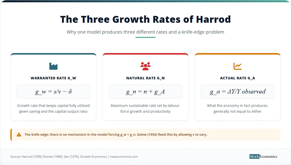
This is the fundamental equation of the Harrod-Domar Growth Model. It defines the warranted rate of growth, denoted \( g_w \). Including a constant depreciation rate, \( \delta \), modifies the equation slightly, because some investment merely replaces worn-out capital rather than adding to the net capital stock:
The warranted rate is the growth rate that keeps the capital stock fully utilised. It is the rate at which the economy must grow to absorb the new capacity created by investment. If the economy grows faster than \( g_w \), demand outstrips capacity. If it grows slower than \( g_w \), capacity outstrips demand, and firms accumulate unsold inventories.
Harrod separately defined the natural rate of growth, denoted \( g_n \). This is the maximum growth rate the economy can sustain, given the growth of the labour force and the growth of labour productivity. Let \( n \) be the growth rate of the labour force and \( g_A \) be the growth rate of labour-augmenting technology. The natural rate is:
The natural rate is a supply-side constraint. It is the rate at which the economy can grow without generating inflation from labour shortages. The third rate is the actual rate of growth, \( g_a \), which is simply the observed GDP growth rate at any given time.
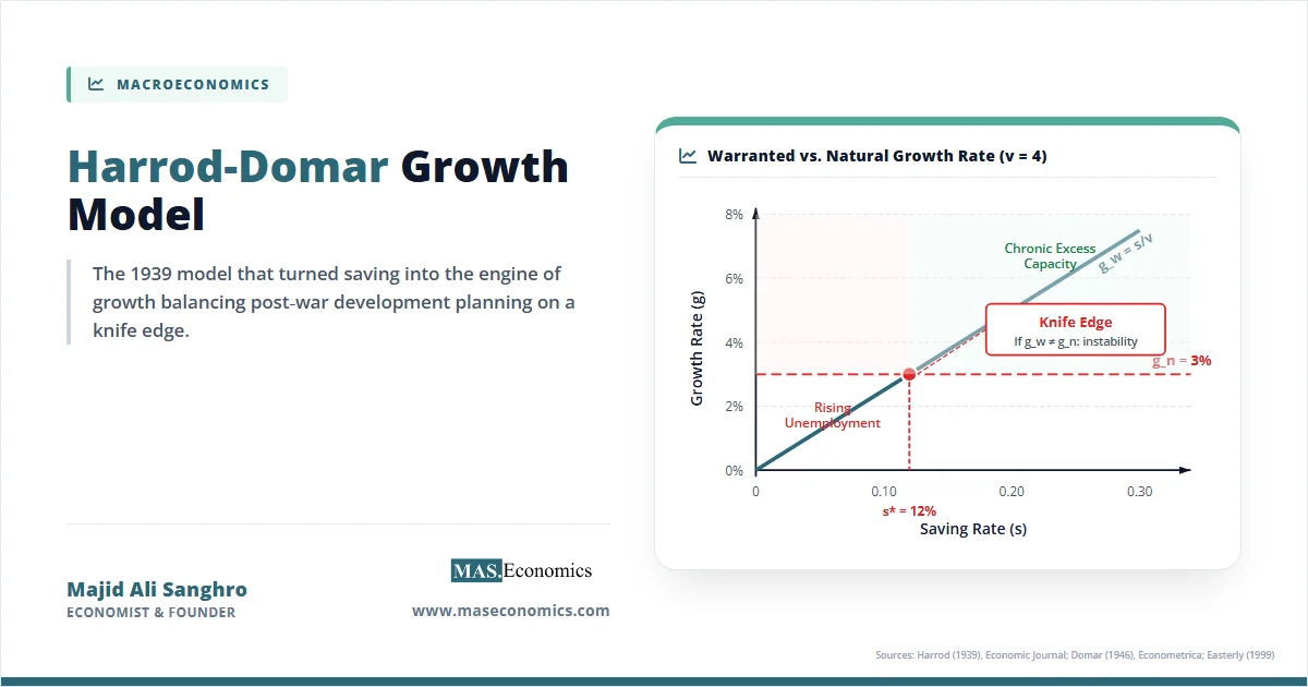
Consider a worked example. Suppose an economy has a saving rate of 0.20, meaning it saves twenty percent of its income. The capital-output ratio is 4, meaning four units of capital are required to produce one unit of output. These figures are commonly cited for post-war industrialised economies. The warranted growth rate is 0.20 divided by 4, which equals 0.05, or five percent per year. Now suppose the labour force grows at two percent per year, and productivity grows at one percent per year. The natural rate of growth is three percent. The warranted rate is higher than the natural rate by two percentage points. The economy tries to grow at five percent, but the labour force only expands at three percent. The result is chronic excess capacity, because firms cannot find the workers needed to operate their new factories, and output falls below the warranted path. The two rates would coincide only at the saving rate \( s^* = v \cdot g_n = 4 \cdot 0.03 = 0.12 \), or twelve percent. At any other saving rate, that gap must close through some mechanism the model does not provide. This is the precise sense in which growth is balanced on a knife-edge.
| Symbol | Name | Definition | Typical Value |
|---|---|---|---|
| \( Y \) | Output | National income / GDP | – |
| \( K \) | Capital stock | Productive capital | – |
| \( s \) | Saving rate | Saving / income | 0.10–0.30 |
| \( v \) | Capital-output ratio | \( K / Y \) | 2–5 |
| \( \delta \) | Depreciation rate | Annual capital decay | 0.05–0.10 |
| \( g_w \) | Warranted growth rate | \( s/v – \delta \) | 2–6% |
| \( g_n \) | Natural growth rate | \( n + g_A \) | 1–4% |
| ICOR | Incremental capital-output ratio | \( \Delta K / \Delta Y \) | 3–6 |
 |
|||
Key Assumptions and Limitations
The Harrod-Domar Growth Model rests on four central assumptions. First, it assumes fixed coefficients in production. The capital-output ratio \( v \) and the labour-output ratio \( u \) are constants. Firms cannot substitute labour for capital when labour becomes expensive, nor capital for labour when capital becomes expensive. This fixed-proportion assumption is the source of the model’s most famous pathology, the knife-edge instability.
Second, the model assumes a constant saving rate. Households and firms always save the same fraction of their income, regardless of the interest rate, the level of income, or expectations about the future. This simplifies the algebra, but it ignores the possibility that saving behaviour might adjust to stabilise the economy. The Ramsey optimal saving framework later showed how households can adjust their saving rate in response to changes in the real interest rate, providing a stabilising mechanism absent in Harrod-Domar.
Third, the basic version of the model assumes a constant capital-output ratio. This implies there is no technological change that alters the amount of capital required to produce a unit of output. In reality, technological progress can be capital-saving, labour-saving, or neutral, and it continuously shifts the capital-output ratio over time.
Fourth, the model assumes a closed economy without government. There are no imports, no exports, no taxes, and no government spending. This assumption isolates the relationship between saving, investment, and growth, but it abstracts from the open-economy dynamics that dominate small, trade-dependent nations.
These assumptions create severe limitations. The most famous is the knife-edge problem. The model provides no mechanism forcing the warranted rate \( g_w \) to equal the natural rate \( g_n \). The warranted rate depends on the saving rate and the capital-output ratio. The natural rate depends on population growth and technological progress. These are determined by entirely different forces. If \( g_w \) exceeds \( g_n \), the economy tries to grow faster than the labour force can support. Firms invest, but they cannot find enough workers to operate the new capital. Capacity goes unused, profits fall, and investment collapses. The economy spirals into a slump. If \( g_w \) falls short of \( g_n \), the labour force grows faster than capital accumulation. Unemployment rises persistently. The economy cannot absorb its own labour supply.
The dynamics of this knife-edge are self-reinforcing, which is what makes the instability so dangerous. Consider a scenario where the actual growth rate \( g_a \) falls slightly below the warranted rate \( g_w \). Because the economy is growing slower than the warranted rate, the new capital stock is not being fully utilised. Firms observe excess capacity. Their natural response is to cut back on new investment orders. Cutting investment, however, reduces aggregate demand through the Keynesian multiplier. Lower demand means even less output is sold, which worsens the excess capacity problem. Firms then cut investment even further. The economy accelerates away from the warranted path downward, not toward it. The same logic applies in reverse. If \( g_a \) exceeds \( g_w \), firms experience a shortage of capacity. They increase investment, which boosts demand further, tightening the capacity constraint even more. Inflation accelerates. The model offers no automatic stabiliser to push the economy back to the narrow equilibrium path.
The empirical failure of the fixed capital-output ratio also limits the model. Nicholas Kaldor later documented his stylised facts of economic growth, showing that the capital-output ratio is roughly stable in the long run but variable cyclically. The assumption of a rigidly constant \( v \) fails to capture how firms adapt their production techniques in response to changing factor prices. Robert Solow’s 1956 model showed that allowing factor substitution, where firms can choose between capital-intensive and labour-intensive techniques, eliminates the knife-edge entirely. When capital accumulates faster than labour, the return on capital falls, and firms naturally shift to more capital-intensive methods, raising the capital-output ratio and slowing the warranted rate down to the natural rate. This process, central to the Solow-Swan growth model, is entirely absent from Harrod-Domar.
Empirical Evidence for Harrod‑Domar
Empirical testing has repeatedly exposed the shortcomings of the Harrod-Domar Growth Model, and especially its central prediction that higher investment automatically yields higher growth. Three studies stand out for their rigour and influence.
William Easterly published “The Ghost of Financing Gap: Testing the Growth Model Used in the International Financial Institutions” in the Journal of Development Economics in 1999. Easterly tested the core Harrod-Domar mechanism used by the World Bank and the International Monetary Fund, in which foreign aid fills a financing gap to boost investment, which in turn boosts growth. He examined data from 88 countries between 1965 and 1995. The Harrod-Domar prediction is straightforward: aid should increase investment, and investment should increase growth. Easterly found that fewer than 6 of the 88 countries showed the predicted positive relationship between aid and investment. The aid simply did not translate into capital accumulation. Much of the foreign aid was consumed rather than invested. Governments used the inflows to finance current consumption, to pay off existing debt, or to import luxury goods. In many cases, aid flows were siphoned off through corruption, enriching elites rather than building factories. The implied capital-output ratios required to make the model fit the data were also wildly unstable, contradicting the model’s foundational assumption of a constant \( v \). Easterly concluded that the financing-gap approach was a statistical illusion and that the Harrod-Domar mechanism was not operating in the real world.
Robert King and Ross Levine documented similar failures in “Capital Fundamentalism, Economic Development, and Economic Growth”, published in the Carnegie-Rochester Conference Series on Public Policy in 1994. They explicitly tested the assumption of a constant incremental capital-output ratio, or ICOR. The ICOR measures how much additional capital is needed to produce an additional unit of output. Harrod-Domar assumes this ratio is stable. King and Levine showed that the ICOR varies wildly across countries and over time, by factors of two to ten. A country shifting from agriculture to light manufacturing might see its ICOR drop as output surges with relatively little new capital. A country building massive but inefficient heavy industries might see its ICOR spike as capital is absorbed into projects that yield low returns. This variation destroys the predictive power of the model, because planners cannot simply divide a target growth rate by a fixed ICOR to determine the required investment. The assumption of constant \( v \) is empirically false.
The most famous empirical critique came from Robert Solow himself in “Technical Change and the Aggregate Production Function”, published in the Review of Economics and Statistics in 1957. Solow used data from the United States covering the period from 1909 to 1949. He decomposed the growth of output per worker into the portion attributable to capital deepening and the portion attributable to total factor productivity, which he called technical change. Total factor productivity, or TFP, is the efficiency with which an economy combines labour and capital to produce output. It captures technological innovation, better management practices, improvements in education, and stronger institutions that allow the same inputs to yield more output. Solow found that 87.5 percent of the growth in output per worker came from total factor productivity, not from capital deepening. This result directly undermines the Harrod-Domar emphasis on \( s/v \) as the engine of growth. If capital accumulation explains only twelve percent of the growth in living standards, then a model that attributes all growth to capital accumulation is missing the most important part of the story. Innovation and efficiency gains, not sheer physical accumulation, are the primary drivers of prosperity.

When the saving rate exceeds 12%, the warranted rate exceeds the natural rate and chronic excess capacity emerges. When it falls below, unemployment grows without bound. Source: Harrod (1939), Economic Journal; Domar (1946), Econometrica; MASEconomics calculation.
How the Harrod‑Domar Model Matters
Despite its theoretical flaws and empirical failures, the Harrod-Domar Growth Model is one of the most influential frameworks in the history of economic thought. Its influence persists because it offers a simple, actionable formula for policymakers. The model tells planners exactly what they must do to raise growth: increase the saving rate or lower the capital-output ratio. This clarity made it the default tool of development planning for three decades.
Development planning in the 1950s and 1960s relied almost entirely on Harrod-Domar logic. The World Bank and national planning commissions used the model to calculate investment requirements. A country that wanted to grow at six percent per year, and had an estimated capital-output ratio of three, simply calculated that it needed an investment rate of eighteen percent of GDP. If domestic savings were only twelve percent of GDP, the financing gap was six percent. Planners then filled that gap with foreign aid or foreign borrowing. This arithmetic defined the structure of international development assistance for a generation.
India’s First Five-Year Plan (1951–1956) is the canonical example. The plan was designed by K.N. Raj using an explicit Harrod-Domar framework. Raj set a target growth rate of 2.1 percent, divided by an assumed capital-output ratio, and arrived at the required investment rate. The plan focused on agriculture, irrigation, and power, sectors with relatively low ICORs. Actual growth came in at 3.6 percent, exceeding the target, which gave Indian planners enormous confidence in the model. The Second Plan (1956–1961), designed by P.C. Mahalanobis, pivoted to heavy industry using the distinct two-sector Feldman-Mahalanobis model, but the underlying logic of saving-driven, investment-led growth remained fundamentally Harrod-Domar in spirit. The results of the Second Plan were mixed. India did build a heavy industrial base, but it also suffered from chronic inefficiencies. Capital was tied up in massive state-owned enterprises that produced steel and machinery regardless of actual demand, leading to severe underutilisation of capacity. Meanwhile, the consumer goods sector and agriculture were starved of investment, leading to food shortages and inflation. The persistent unemployment and idle factories were a direct manifestation of the knife-edge problem the model could not solve.
Aid-financing-gap thinking dominated international institutions through the 1990s. United Nations documents and IMF reports routinely set country aid envelopes by computing the gap between domestic savings and the investment required at a target growth rate, divided by an assumed ICOR. Easterly’s 1999 critique dismantled this practice. He showed that aid did not reliably increase investment, and that investment did not reliably increase growth. The implied ICORs were unstable, and the entire exercise rested on a logical fallacy: the assumption that a correlation between investment and growth implies that causing investment will cause growth. After Easterly, the World Bank and the IMF quietly abandoned strict Harrod-Domar targeting, though the intellectual habits persist.
Modern relevance is surprisingly strong. Capital fundamentalism survives in infrastructure-led growth strategies. China’s 2008 stimulus programme, which deployed four trillion yuan into roads, railways, and housing, relied on the implicit assumption that capital accumulation drives growth. The stimulus did boost short-run demand, but it also left China with vast excess capacity in heavy industry and real estate. Entire “ghost cities” were built with new apartments and roads but no residents. The steel and cement sectors expanded far beyond what the domestic economy could absorb, creating a classic Harrod-Domar imbalance where the warranted rate outstripped the natural rate. The overcapacity was so severe that Chinese policymakers later had to force cuts in industrial production. The African Development Bank’s High 5 strategy, which prioritises infrastructure investment, also relies on Harrod-Domar logic. The strategy assumes that filling Africa’s infrastructure gap will automatically translate into higher growth, a bet that depends on a stable ICOR that history does not guarantee.
Debates over the European Union’s NextGenerationEU programme echo the same themes. The programme was designed to fund massive public investment in green and digital infrastructure across Europe. Proponents argued that low interest rates and high saving rates meant the warranted rate exceeded the natural rate, creating a savings glut that public investment could absorb. Opponents warned that poorly targeted investment would merely inflate asset prices or fund low-productivity projects, raising the capital-output ratio and yielding little growth. Both sides were arguing within the Harrod-Domar framework, even if they did not name it.
The Harrod-Domar Growth Model is also important because of what it provoked. Its knife-edge instability directly motivated Robert Solow and Trevor Swan to build a better model. Solow’s 1956 paper introduced the Cobb-Douglas production function, which allows continuous substitution between capital and labour. When capital accumulates faster than labour, the marginal product of capital falls, and firms naturally substitute toward labour-intensive techniques. This substitution raises the capital-output ratio and slows the warranted rate until it converges with the natural rate. The knife-edge disappears. Growth is stable. The Solow-Swan model replaced Harrod-Domar as the standard framework for analysing long-run growth, precisely because it solved the instability problem that Harrod and Domar had uncovered.
However, the Solow-Swan model created a new problem. By making growth stable, it made the saving rate irrelevant to long-run growth. In the Solow model, a higher saving rate raises the level of output per capita but does not change the long-run growth rate, which is determined entirely by the exogenous rate of technological progress. Endogenous growth theory, developed by Paul Romer and others in the 1980s and 1990s, challenged this result. Romer’s endogenous growth theory argued that ideas and knowledge are non-rival goods that can generate increasing returns to scale at the aggregate level. Because knowledge does not suffer from diminishing returns in the same way physical capital does, a higher saving rate can permanently increase the growth rate if the saved resources are invested in research and development. In this sense, endogenous growth theory restored a role for saving that Harrod-Domar had asserted, but Solow had denied, though it did so through a completely different mechanism.
The model is wrong on the mechanism, but right that without investment, there is no growth. Modern empirical studies still use ICOR-style accounting as a first approximation. Economists at the IMF and the World Bank still compute incremental capital-output ratios to assess whether investment is productive. The ICOR is a rough measure, but it gives a quick sanity check on growth projections. If a country claims it will grow at eight percent with an investment rate of twenty percent and an ICOR of three, the arithmetic is at least consistent. If the same country claims it will grow at eight percent with an investment rate of fifteen percent, the implied ICOR is too low to be plausible, and the projection is almost certainly wrong. This diagnostic power is the Harrod-Domar Growth Model’s enduring practical legacy.
MASEconomics Explains
4 economic concepts behind the Harrod-Domar Growth Model
Conclusion
The Harrod-Domar Growth Model is the first formal long-run growth theory and the direct ancestor of every later model in the field. It defines a warranted rate, a natural rate, and an actual rate, but contains no mechanism to align them. The resulting knife-edge instability means economies either accumulate excess capacity or suffer rising unemployment. Empirical work from Easterly to Solow has largely rejected its constant capital-output ratio and its financing-gap logic, even as development planners continue to use its basic arithmetic.
Did you find this article helpful? Share it with someone who loves economics. And remember, at MASEconomics, we make complex ideas simple.