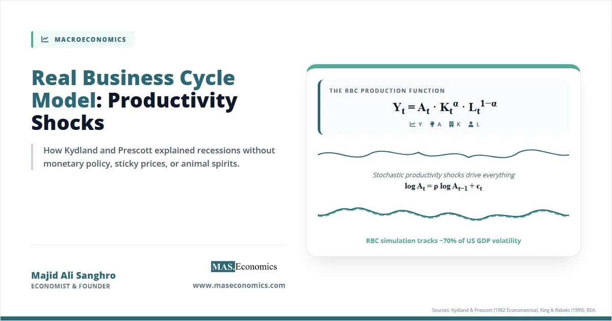
The real business cycle model explains aggregate fluctuations as the optimal response of forward-looking households and competitive firms to exogenous total factor productivity shocks, dispensing with monetary policy and nominal frictions as drivers of recessions. Introduced by Finn Kydland and Edward Prescott in their 1982 Econometrica paper “Time to Build and Aggregate Fluctuations,” this framework made a radical claim: business cycles are not failures of the price system requiring government intervention. Instead, fluctuations represent the efficient allocation of resources in response to real shocks. This claim challenged the entire Keynesian paradigm that had dominated macroeconomic policy since the 1940s.
The Logic of Real Business Cycles
Before the 1980s, macroeconomic theory viewed business cycles and economic growth as separate subjects. Growth theory, anchored by the Solow-Swan growth model, explained long-run trends through capital accumulation and technological progress. Business cycle theory, dominated by Keynesian models, explained short-run fluctuations through demand shocks, sticky prices, and monetary surprises. The two literatures rarely interacted. Kydland and Prescott demolished this separation. They built a stochastic version of the Solow growth model, added intertemporal labour-leisure choices, and demonstrated that random productivity shocks alone could generate fluctuations statistically indistinguishable from post-war US business cycles.
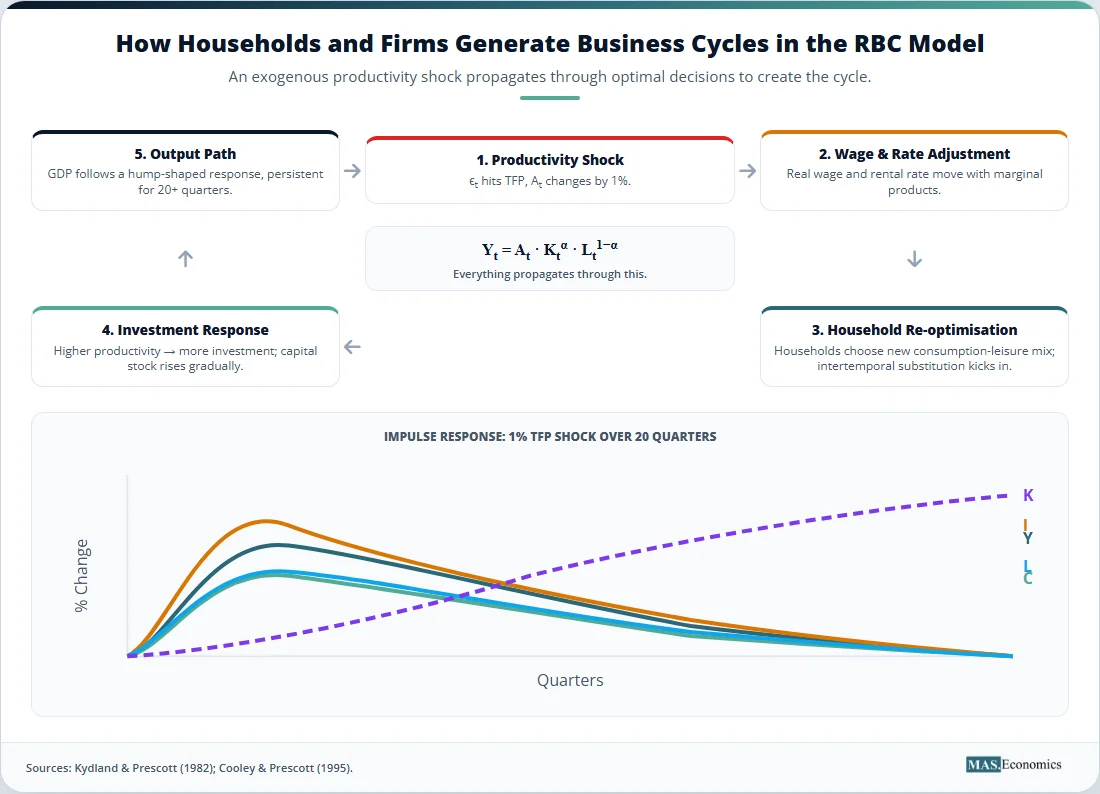
The model’s logic rests on intertemporal substitution. When a positive productivity shock hits, the real wage rises because workers become more productive. Forward-looking households recognise that current wages are high relative to future expected wages, so they work more today and less in the future. They also save more of their current income, increasing investment. When a negative productivity shock hits, the process reverses: households work less and save less. The observed recession is not a market failure; it is the rational, welfare-maximising response to a temporary deterioration in production possibilities.
This framework contains no role for monetary policy. Prices and wages adjust instantaneously to clear markets. Money is neutral, affecting only nominal variables. Recessions occur because technology has temporarily regressed, making the economy genuinely poorer. Attempting to stabilise these fluctuations through fiscal or monetary stimulus would distort the optimal consumption and labour choices of rational agents, potentially reducing welfare rather than enhancing it.
The methodological revolution was as important as the theoretical one. Kydland and Prescott replaced traditional econometric estimation with calibration. Instead of fitting the model to business cycle data using statistical techniques, they chose parameter values based on long-run averages and microeconomic studies, then asked whether the calibrated model could replicate key statistical properties of the actual economy. This approach shifted the profession toward computational experiments and formal dynamic general equilibrium modelling. Prescott’s 2004 Nobel Prize, shared with Kydland, explicitly recognised this methodological transformation.
RBC Model in Equations
The baseline real business cycle model derives aggregate fluctuations from the optimising behaviour of a representative household and a representative firm in a perfectly competitive, stochastic environment.
Household Problem
A representative household maximises discounted expected utility over consumption \( C_t \) and leisure \( 1 – L_t \), where \( L_t \) is the fraction of time spent working:
subject to the budget constraint:
where \( I_t \) is investment, \( w_t \) is the real wage, and \( r_t \) is the rental rate of capital. The parameter \( \beta \in (0,1) \) is the subjective discount factor, reflecting the household’s preference for present over future consumption. Utility functions typically take the form \( U(C, 1-L) = \log C + \phi \log(1-L) \), which yields closed-form solutions for the steady state and simplifies the log-linearisation around it.
Capital Accumulation
The household accumulates capital according to the law of motion:
where \( \delta \) is the depreciation rate. The time-to-build specification in the original Kydland-Prescott paper introduced lags between investment decisions and capital installation, generating richer dynamics than the standard one-period adjustment assumption.
Production Technology
A representative firm produces output using a Cobb-Douglas production function:
where \( A_t \) is total factor productivity (TFP) and \( \alpha \) is the capital share of income. Under perfect competition, factors are paid their marginal products: the real wage equals the marginal product of labour, and the rental rate equals the marginal product of capital.
Stochastic Productivity Process
The sole driving force of fluctuations is the exogenous productivity shock, modelled as a first-order autoregressive process:
The persistence parameter \( \rho \) governs how long productivity shocks last. The standard deviation \( \sigma_\varepsilon \) governs their magnitude. These shocks, often proxied by the Solow residual in empirical work, are the engine of the business cycle in this framework.
Equilibrium Conditions
The competitive equilibrium is characterised by the Euler equation governing consumption smoothing, the intratemporal condition linking consumption and labour supply, the capital accumulation equation, and the aggregate resource constraint \( Y_t = C_t + I_t \). Dynamic programming techniques solve this system, typically by log-linearising around the deterministic steady state.
Key Quantitative Implication
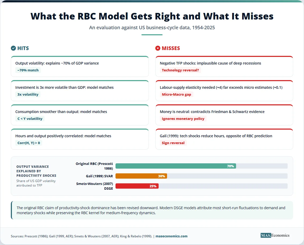
When the calibrated model is fed actual Solow residuals as input, the simulated path of output tracks the data closely. Prescott (1986) showed that the baseline specification explains about 70% of US output volatility. This dramatic result was the primary evidence supporting the real business cycle approach: a model with only one shock could replicate most of the observed variation in aggregate output.
Key Assumptions and Limitations
The real business cycle model relies on a set of strong assumptions. First, a representative agent with rational expectations makes all consumption and labour decisions. Second, perfect competition and complete markets ensure that all resources are efficiently allocated at every point in time. Third, prices and wages adjust instantaneously, so markets always clear. Fourth, productivity shocks are the dominant driver of economic fluctuations.
These assumptions generate significant limitations. First, the Solow residual is poorly measured. The Solow residual captures everything not explained by measured capital and labour inputs, including measurement error, capacity utilisation variations, and labour hoarding during recessions. King and Rebelo (1999) documented that variations in capacity utilisation alone can account for a substantial fraction of the observed Solow residual variation, meaning that much of what the RBC model treats as technology shocks may simply reflect firms adjusting how intensively they use existing capital.
Second, the model requires implausibly large negative productivity shocks to explain deep recessions. The 2008 financial crisis saw US output fall sharply, but attributing this entirely to a sudden forgetfulness of technology strains credulity. Firms did not suddenly forget how to produce; rather, financial frictions disrupted the allocation of capital and labour.
Third, the model abstracts entirely from monetary policy. Friedman and Schwartz (1963) demonstrated that monetary contractions precede most major depressions, a finding the RBC framework simply ignores by assuming money is neutral even in the short run.
Fourth, the labour-supply elasticity required to match the observed volatility of hours worked is far higher than microeconomic evidence supports. The standard model requires an elasticity of around 4, while microeconometric studies typically find values closer to 0.1. Hansen (1985) addressed this by introducing indivisible labour, where households either work a fixed shift or do not work at all, effectively aggregating individual lotteries into a higher aggregate elasticity. While ingenious, this assumption remains controversial because it departs from the smooth optimisation at the model’s core.
Fifth, the model cannot explain the procyclicality of price-cost markups. If markets are perfectly competitive, markups are constant by assumption. Empirical evidence shows markups are countercyclical, rising during recessions when firms with market power maintain prices while costs fall. This observation points to nominal rigidities and imperfect competition, both absent from the RBC framework.
Sixth, the model ignored the role of credit and finance. The 2008 crisis exposed this omission starkly: financial intermediation collapsed, credit dried up, and investment plummeted. A framework that treats investment as the rational response to productivity shocks cannot explain a recession triggered by a banking panic.
Empirical Evidence for the RBC Model
Kydland and Prescott (1982) demonstrated that their calibrated model could replicate key business cycle moments for the US economy. The model matched the relative volatility of consumption and investment, the procyclicality of hours worked, and the autocorrelation of output. Prescott (1986) famously claimed that the model explained 70% of post-war US output fluctuations, a figure that became the benchmark for evaluating RBC performance.
Long and Plosser (1983) provided independent support with a multi-sector RBC model showing that sector-specific productivity shocks could generate aggregate fluctuations through input-output linkages. Their model explained how idiosyncratic shocks propagate through the economy, creating comovement across sectors without any aggregate shock. Hansen (1985) resolved the labour-volatility puzzle by introducing indivisible labour, bringing the model’s predictions for hours volatility much closer to the data.
The empirical consensus shifted as critics identified fundamental identification problems. Galí (1999) provided the most influential counter-evidence using structural vector autoregressions (SVARs) to identify technology shocks. His key finding: identified positive technology shocks reduce hours worked in the short run, contradicting the RBC prediction that hours should rise. If technology shocks cause hours to fall, they cannot be the primary driver of observed business cycles, where output and hours move together strongly.
Smets and Wouters (2007) estimated a DSGE model with both nominal rigidities and multiple shocks. Their results showed that productivity shocks explain only about 25–35% of US business cycle variance, with demand shocks, monetary policy shocks, and preference shocks accounting for the majority. This finding dramatically reduced the estimated contribution of technology shocks relative to the original RBC claims.
Galí and Rabanal (2004) extended the SVAR analysis to the euro area, finding similarly that technology shocks explain a small fraction of business cycle fluctuations. The forecasting implications are significant: if technology shocks are not the primary driver, models that focus exclusively on them will misidentify the sources of fluctuations and prescribe inappropriate policy responses.
Sources: King & Rebelo (1999); BEA; Penn World Tables; baseline calibration follows Cooley & Prescott (1995).
| Parameter | Symbol | Value | Source / Justification | Empirical Match |
|---|---|---|---|---|
| Capital share | \( \alpha \) | 0.36 | US capital income share in NIPA | BEA national accounts |
| Discount factor | \( \beta \) | 0.99 | 4% annualised real interest rate | Real returns on T-bills |
| Depreciation rate | \( \delta \) | 0.025 | 10% annual depreciation | NIPA capital stock |
| Productivity persistence | \( \rho \) | 0.95 | AR(1) coefficient on Solow residual | Quarterly TFP series |
| Productivity innovation std. dev. | \( \sigma_\varepsilon \) | 0.007 | Std. dev. of Solow residual innovations | Quarterly TFP series |
| Labour share of time | \( \bar{L} \) | 0.30 | Avg. fraction of hours worked | CPS / time-use surveys |

|
||||
How the RBC Model Matters
The real business cycle model reshaped macroeconomics in three profound ways: methodologically, theoretically, and institutionally.
The methodological revolution is perhaps the most enduring legacy. Before Kydland and Prescott, macroeconomists estimated reduced-form equations on aggregate data, paying little attention to whether the equations were consistent with microeconomic optimisation. The RBC approach required that every equation in the model be derived from first principles: household utility maximisation, firm profit maximisation, and market clearing. Parameters were calibrated to match long-run averages and microeconomic estimates rather than fitted to business cycle data. This calibration methodology became the standard for modern macroeconomics. Every major central bank now runs DSGE models that descend from the RBC architecture, using the same calibration logic that Kydland and Prescott pioneered.
Theoretically, the RBC model established the stochastic dynamic general equilibrium framework as the lingua franca of macroeconomics. The models built by the ECB, the Federal Reserve, the Bank of England, and the Bank of Canada all use the RBC kernel as their “real” core, layered with nominal rigidities, financial frictions, and policy rules. Monetary policy analysis today is conducted within models that are genetically RBC at their foundation. Without the RBC contribution, the New Keynesian synthesis that dominates current policy analysis would not exist in its present form.
The 2004 Nobel Prize confirmed the framework’s significance. The Royal Swedish Academy of Sciences awarded the prize to Kydland and Prescott for “their contributions to dynamic macroeconomics: the time consistency of economic policy and the driving forces behind business cycles.” The citation explicitly recognised both the time-consistency work and the RBC methodology.
Productivity-shock interpretations of post-2008 stagnation illustrate the model’s continued relevance. Fernald (2014) showed that US productivity growth slowed sharply after 2004, well before the financial crisis. This finding suggests that part of the slow recovery reflected a real structural slowdown rather than purely demand deficiency. The RBC logic implies that if potential output has grown more slowly, GDP growth will remain subdued regardless of monetary or fiscal stimulus. Distinguishing between demand-driven and supply-driven slowdowns is critical for policy design, and the RBC framework provides the theoretical apparatus for doing so.
The COVID-19 pandemic provided a striking case study. The 2020 collapse in output fit the RBC logic better than purely demand-driven Keynesian models. Lockdowns directly restricted supply: firms could not produce, workers could not work, and productivity fell sharply. This was a massive, observable negative productivity shock. While the subsequent recovery involved significant demand-side dynamics and monetary accommodation, the initial impetus was real. The pandemic demonstrated that the RBC framework captures a class of shocks that purely nominal models miss. The AI productivity paradox similarly raises questions about whether technology diffusion constitutes a real shock with delayed macroeconomic effects.
The policy implication of the RBC model is that stabilisation attempts may reduce welfare. If business cycles represent optimal responses to real shocks, then monetary or fiscal interventions that dampen fluctuations distort the signals guiding resource allocation. A household that chooses to work less during a negative productivity shock is responding rationally to a lower real wage; subsidising its income to maintain consumption prevents the efficient adjustment. This argument fed the rules-based policy turn of the 1980s and 1990s, providing intellectual support for the view that monetary policy should follow predictable rules rather than engage in discretionary fine-tuning.
Paradoxically, the RBC model’s empirical weaknesses also propelled the development of the New Keynesian synthesis. The need for implausible negative technology shocks, the weak performance on inflation dynamics, and the assumption of monetary neutrality drove economists to combine the RBC’s microfoundations with nominal rigidities. The resulting New Keynesian DSGE models preserve the RBC structure for real variables while adding sticky prices, wage rigidities, and financial frictions to explain short-run demand effects and monetary transmission.
Climate macroeconomics represents the newest frontier for the RBC framework. Modern climate-RBC models embed weather and emissions shocks into the production function, treating climate change as a persistent negative productivity shock. Rebelo (2005) and others have shown that the standard RBC apparatus can be extended to analyse the macroeconomic costs of climate damage and the welfare effects of carbon taxation. Golosov, Hassler, Krusell, and Tsyvinski (2014) developed a tractable climate-RBC model where a carbon tax equal to the social cost of carbon is the optimal policy. This application demonstrates the model’s flexibility as a quantitative laboratory for policy evaluation.
MASEconomics Explains
4 economic concepts behind the real business cycle model
Conclusion
Real business cycle model theory showed that frictionless models with productivity shocks could replicate major business-cycle moments, introducing calibration as the standard methodology and establishing the stochastic dynamic general equilibrium framework as the foundation of modern macroeconomics. The model remains the real core of the DSGE models used by major central banks, and its logic applies directly to supply-driven recessions like the COVID-19 downturn. However, the framework faces ongoing critiques about the implausibility of large negative technology shocks, the poor measurement of total factor productivity, and its inability to explain the role of demand shocks and financial frictions. These limitations drove the New Keynesian synthesis, which preserved the RBC’s microfoundations while adding the nominal rigidities necessary to explain observed inflation dynamics and monetary policy effects.
Did you find this article helpful? Share it with someone who loves economics. And remember, at MASEconomics, we make complex ideas simple.